Class 11 PCM . Chemistry . Chemistry Part I . Structure of Atom
Chapter 2: Structure Of Atom
Ch 2
Chemistry
Class 11 PCM
Discovery Of Sub-Atomic
From the indivisible atom to subatomic particles
Changing ideas about the atom
- Chemical behaviour: Differences in elements’ chemical behaviour arise from differences in the internal structure of their atoms.
- Early ideas: Around 400 B.C., Indian and Greek philosophers proposed that matter consisted of indivisible particles called atoms; the Greek-derived word means “uncuttable.”
- Dalton’s theory: In 1808, John Dalton put atomic theory on a firm scientific basis and treated atoms as the ultimate particles of matter.
- What it explained: Dalton’s theory successfully explained the laws of conservation of mass, constant composition and multiple proportions.
- Limitation: It could not explain electrical behaviour, such as glass or ebonite becoming charged when rubbed with silk or fur.
- Modern conclusion: Experiments in the late nineteenth and early twentieth centuries established that atoms contain electrons, protons and neutrons.
- Charge rule: Like charges repel; unlike charges attract.
- Faraday (1830): Chemical changes and release or deposition of matter at electrodes during electrolysis supported the particulate nature of electricity.
Discovery of the electron
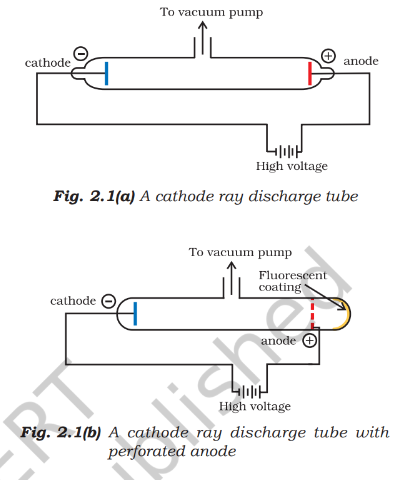
Cathode rays — Streams of particles that travel from the negative cathode towards the positive anode in a gas-discharge tube.
Cathode-ray discharge tube
- Conditions: Discharge through a gas occurs at very low pressure and high voltage in a tube containing two electrodes.
- Detection: The rays are invisible, but fluorescent or phosphorescent materials glow when struck; zinc sulphide behind a perforated anode shows a bright spot.
- Path: Without electric or magnetic fields, cathode rays travel in straight lines.
- Charge: Their deflection in electric and magnetic fields indicates that they are negatively charged particles, called electrons.
- Universal nature: Their properties do not depend on the electrode material or the gas in the tube; electrons are constituents of all atoms.
- Application: Television picture tubes use cathode rays to produce fluorescence on the screen.
Charge-to-mass ratio of the electron
J. J. Thomson’s measurement
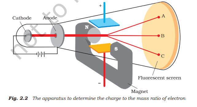
- Date and method: In 1897, J. J. Thomson passed electrons through mutually perpendicular electric and magnetic fields, both perpendicular to the beam.
- Deflection: An electric field alone or a magnetic field alone deflects the beam; balancing their strengths restores its undeflected path.
- Factors: Deflection increases with particle charge and field strength, and increases as particle mass decreases.
- Result: Thomson measured the magnitude of the electron’s charge-to-mass ratio.
Here, is the magnitude of the electron charge and is its mass; the electron itself carries charge .
Charge and mass of the electron
Millikan’s oil-drop experiment
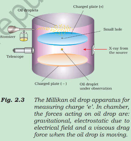
- Date: R. A. Millikan carried out the oil-drop experiment during 1906–1914.
- Method: Charged oil droplets between condenser plates were observed as the electric field was varied to retard, accelerate or suspend their motion.
- Quantisation: Each droplet’s charge was an integral multiple of the elementary charge: , where .
- Millikan’s result: He found the electron charge to be ; the present accepted value is .
How the oil-drop measurement works
- Fine oil droplets enter the space between condenser plates and acquire charge by colliding with ions in the air.
- Observe their motion through a telescope with a micrometer eyepiece; the rate of fall is used to determine droplet mass.
- Vary the electric field and measure its effect on the motion of the charged droplets.
- The charge on each droplet is a whole-number multiple of the elementary charge.
Combining Millikan’s accepted electron-charge magnitude with Thomson’s ratio gives the electron mass.
Discovery of protons and neutrons
Positive canal rays and the proton
- Canal rays: Electrical discharge in a modified cathode-ray tube produced positively charged particles called canal rays.
- Nature: These are positive gaseous ions; their mass and charge-to-mass ratio depend on the gas from which they originate.
- Charge and field behaviour: Some carry multiple units of the fundamental charge and behave oppositely to electrons in electric or magnetic fields.
- Proton: The smallest and lightest positive ion, obtained from hydrogen, is the proton; it was characterised in 1919.
Neutron
- Discovery: In 1932, James Chadwick bombarded a thin sheet of beryllium with alpha particles.
- Identification: The emitted electrically neutral particles had a mass slightly greater than that of protons; Chadwick named them neutrons.
| Particle | Symbol | Absolute charge (C) | Relative charge | Mass (kg) | Mass (u) | Approximate mass (u) |
|---|---|---|---|---|---|---|
| Electron | ||||||
| Proton | ||||||
| Neutron |
What evidence showed that cathode rays consist of electrons?
How were the electron’s charge and mass determined?
How were the proton and neutron identified?
Quick recap
- Atomic structure: Differences in elements’ chemical behaviour reflect differences in their atoms’ internal structures.
- Dalton (1808): Explained conservation of mass, constant composition and multiple proportions, but not electrical charging by rubbing.
- Electron: Cathode rays are universal, negatively charged particles travelling from cathode to anode.
- Thomson (1897): Measured .
- Millikan (1906–1914): Found electron charge ; the accepted value is .
- Electron mass: Combining charge and charge-to-mass ratio gives .
- Proton and neutron: The hydrogen positive ion is the proton (characterised in 1919); Chadwick discovered the neutral neutron in 1932.
Atomic Models
Why Atomic Models Were Needed
Problems to Explain
- Atomic structure: Explain how positive and negative subatomic particles are arranged inside the atom.
- Stability: Explain why atoms remain stable.
- Properties and molecules: Relate atomic structure to the physical and chemical properties of elements and the formation of molecules.
- Radiation: Explain the origin and nature of electromagnetic radiation absorbed or emitted by atoms.
Thomson Model of the Atom
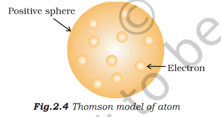
Thomson model — An atomic model in which electrons are embedded in a sphere of uniformly distributed positive charge.
Key Features
- Proposed: J. J. Thomson proposed the model in 1898.
- Shape and size: The atom was described as a sphere with radius about .
- Arrangement: Positive charge fills the sphere uniformly; electrons are embedded in a stable electrostatic arrangement.
- Names: Also called the plum-pudding, raisin-pudding or watermelon model.
X-Rays and Radioactivity
X-Rays
- Discovery: In 1895, Wilhelm Röntgen found that rays were produced when electrons struck a material in a cathode-ray tube; he named them X-rays.
- Production: They are produced effectively when electrons hit a dense metal target (anode).
- Properties: X-rays are electromagnetic, have very short wavelengths of about , are not deflected by electric or magnetic fields, and have high penetrating power.
- Use: Their ability to pass through matter makes them useful for examining the interiors of objects.
Radioactivity — The spontaneous emission of radiation by certain elements, called radioactive elements.
| Radiation | Nature and charge | Penetrating power |
|---|---|---|
| -rays | High-energy particles; charge , mass about ; helium nuclei | Lowest |
| -rays | Negatively charged particles similar to electrons | About 100 times that of -rays |
| -rays | Neutral, high-energy electromagnetic radiation; not particles | About 1000 times that of -rays |
Radiation Notes
- Alpha particles: Rutherford identified them as helium nuclei; gaining two electrons produces a helium atom.
- Research: The study of radioactivity was developed by Marie Curie, Pierre Curie, Rutherford and Frederick Soddy.
Rutherford’s Gold-Foil Experiment
Experiment and Results
- Experiment: Rutherford, with Hans Geiger and Ernest Marsden, directed alpha particles at a very thin gold foil.
- Thomson-model expectation: If mass and positive charge were spread uniformly, alpha particles should pass through with only slight slowing or small deflections.
- Observation 1: Most alpha particles passed through undeflected.
- Observation 2: A small fraction was deflected through small angles.
- Observation 3: A very small fraction—about 1 in 20,000—bounced back, deflected by nearly .
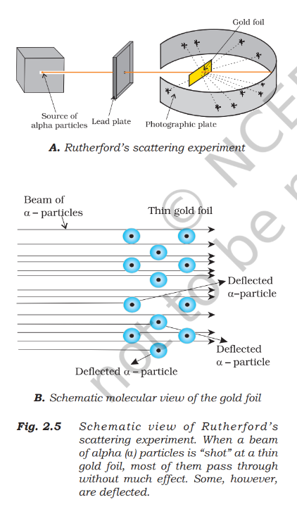
| Observation | Conclusion |
|---|---|
| Most alpha particles pass through undeflected. | Most of the atom is empty space. |
| Some positively charged alpha particles are deflected. | The atom’s positive charge is concentrated in a small region that repels them. |
| A very small number bounce back. | The positive region is extremely small and dense; it contains most of the atom’s mass. |
Relative Sizes
- Atom radius: About .
- Nucleus radius: About ; its volume is negligible compared with the atom’s volume.
- Scale analogy: If a cricket ball represented the nucleus, the atom would have a radius of about .
Rutherford’s Nuclear Model
Nucleus — The extremely small, dense central region of an atom, containing its positive charge and most of its mass.
Model Features
- Central nucleus: Positive charge and most of the atom’s mass are concentrated in the nucleus.
- Electrons: Electrons move rapidly around the nucleus in circular paths called orbits.
- Attraction: Electrostatic forces of attraction hold electrons and the nucleus together.
- Solar-system analogy: The nucleus is like the Sun, while orbiting electrons are like planets.
| Point | Thomson model | Rutherford model |
|---|---|---|
| Positive charge | Spread uniformly through the atom | Concentrated in a tiny nucleus |
| Electrons | Embedded in the positive sphere | Move around the nucleus in orbits |
| Space in atom | Not described as mostly empty | Mostly empty space |
What did Rutherford conclude from the gold-foil experiment?
Why were a few alpha particles deflected or sent back?
Quick recap
- Thomson’s model places electrons inside a uniformly positively charged sphere.
- X-rays are penetrating electromagnetic radiation; radioactive elements emit alpha, beta and gamma radiation.
- Alpha particles are high-energy helium nuclei with charge and mass about .
- Most alpha particles pass through gold foil, but a few are deflected and very few bounce back.
- Rutherford concluded that atoms are mostly empty space with a tiny, dense, positively charged nucleus.
- Electrons orbit the nucleus and are held by electrostatic attraction.
Atomic Number and Mass Number
Atomic Number and Mass Number
Nuclear charge and atomic number
- Nuclear charge: The nucleus is positively charged because it contains protons; a proton’s charge is equal in magnitude and opposite in sign to an electron’s charge.
- Atomic number (): The number of protons in the nucleus; in a neutral atom, it also equals the number of electrons.
- Examples: Hydrogen has and sodium has ; neutral atoms of these elements contain and electrons respectively.
For a neutral atom, the proton and electron counts are equal.
Mass number () — The total number of protons and neutrons (nucleons) in an atom’s nucleus.
The neutron count is found by subtracting the atomic number from the mass number; this applies to atoms and ions.
Representing an atom or ion
- Notation: Write a species as ; is the mass number and is the atomic number.
- Neutral atom: The numbers of protons and electrons are equal.
- Ion: More protons than electrons means a cation; fewer protons than electrons means an anion.
Isobars and Isotopes
| Isobars | Isotopes | |
|---|---|---|
| Same quantity | Mass number, | Atomic number, |
| Different quantity | Atomic number, | Mass number, ; therefore, neutron count differs |
| Example | and | Hydrogen isotopes: , , |
Examples and chemical behaviour of isotopes
- Hydrogen: Protium, , makes up of hydrogen atoms; deuterium, , makes up ; tritium, , occurs only in trace amounts on Earth.
- Carbon: , and contain , and neutrons respectively.
- Chlorine: and contain and neutrons respectively.
- Chemical properties: Isotopes have similar chemical behaviour because they have the same proton number and, as neutral atoms, the same electron number; neutrons have little effect on chemical properties.
Finding particles in an atom or ion
- Bromine-80: For neutral , protons , electrons , and neutrons .
- Sulphur ion: A species with protons, neutrons and electrons has and . Its charge is , so its symbol is .
Do not assume electrons equal protons for ions: first identify whether the species is neutral, a cation or an anion. Neutrons always equal .
Drawbacks of Rutherford’s Model
Solar-system analogy and forces
- Analogy: Rutherford’s model pictures the nucleus as a massive sun and electrons as lighter planets in well-defined orbits.
- Gravity: The force between two masses follows an inverse-square relation, where is the gravitational constant.
- Coulomb force: The force between charged particles has a similar inverse-square form; this resemblance suggests planet-like electron orbits.
Here, and are masses, is their separation, and is the gravitational constant.
Here, and are charges, is their separation, and is the proportionality constant.
Why Rutherford’s model predicts an unstable atom
- The model pictures electrons moving in planet-like orbits around the nucleus.
- An orbiting electron is accelerated because its direction continually changes, even if its speed is constant.
- Maxwell’s electromagnetic theory says an accelerated charged particle emits electromagnetic radiation.
- Radiation carries away the electron’s energy, so its orbit should shrink and it should spiral into the nucleus in about .
- Atoms do not collapse this way; therefore, Rutherford’s model cannot explain atomic stability.
Other limitations
- Stationary electrons do not solve the problem: Electrostatic attraction would pull them into the nucleus.
- Unexplained structure: The model does not describe how electrons are distributed around the nucleus or specify their energies.
Developments Leading to Bohr’s Model
Key developments
- Niels Bohr: Used results from radiation–matter interactions to improve Rutherford’s atomic model.
- Dual nature of electromagnetic radiation: Radiation shows both wave-like and particle-like properties.
- Atomic spectra: Experimental results about atomic spectra also contributed to the formulation of Bohr’s model.
How do isotopes of the same element differ, and why do they have similar chemical behaviour?
Why does Rutherford’s model fail to explain atomic stability?
State the two developments that helped lead to Bohr’s model.
Quick recap
- Atomic number is the proton count; in a neutral atom it also equals the electron count.
- Mass number , so the neutron count is .
- Isobars share a mass number; isotopes share an atomic number.
- Isotopes have similar chemical behaviour because their electron arrangements are the same.
- Rutherford’s model predicts electron energy loss and collapse, so it cannot explain atomic stability.
- Bohr’s model was motivated by radiation’s dual nature and evidence from atomic spectra.
Wave Nature Of Electromagnetic Radiation
Thermal Radiation and Electromagnetic Waves
Thermal radiation — Radiation emitted or absorbed by heated objects; it consists of electromagnetic waves of different frequencies and wavelengths.
Nature of electromagnetic waves
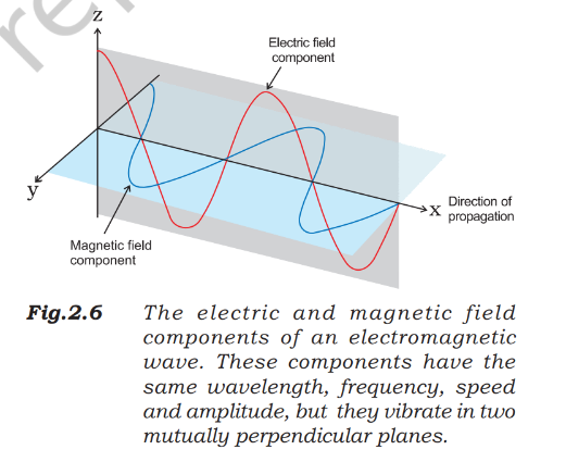
- Maxwell’s explanation: An accelerating charged particle produces changing electric and magnetic fields that travel as electromagnetic waves.
- Light: Light is electromagnetic radiation, with oscillating electric and magnetic fields.
- Confirmation: Maxwell proposed the electromagnetic-wave explanation; Heinrich Hertz later confirmed it experimentally.
Properties and Electromagnetic Spectrum
Key properties
- Perpendicular fields: The electric and magnetic fields are perpendicular to each other and to the direction of propagation.
- No medium needed: Unlike sound or water waves, electromagnetic waves can travel through a vacuum.
Electromagnetic spectrum — The full range of electromagnetic radiations, classified by their different wavelengths or frequencies.
| Region | Approximate frequency | Example use or source |
|---|---|---|
| Radio | Broadcasting | |
| Microwave | Radar | |
| Infrared | Heating | |
| Visible light | Around | The part detected by the human eye |
| Ultraviolet | A component of sunlight |
Detecting radiation
- Visible light is the small part of the electromagnetic spectrum that our eyes can detect.
- Non-visible radiation requires special instruments for detection.
Frequency, Wavelength and Wavenumber
| Quantity | Meaning | Unit |
|---|---|---|
| Frequency, | Number of waves passing a given point per second | Hertz: |
| Wavelength, | Distance between successive corresponding points of a wave | Metre () in SI; smaller length units are also used |
| Wavenumber, | Number of wavelengths per unit length; equal to the reciprocal of wavelength | in SI; is commonly used |
In vacuum, all electromagnetic radiations travel at the same speed, regardless of wavelength.
Relationships and constants
- Speed of light: in vacuum; more precisely, .
- Inverse relationship: Since is constant, increasing frequency means decreasing wavelength, and vice versa.
- Useful rearrangements: and .
Use the reciprocal of wavelength, with wavelength expressed in the corresponding length unit.
A radio station broadcasts at . Find its wavelength and identify the spectrum region.
What frequency range corresponds to visible wavelengths from to ?
Find the wavenumber and frequency of yellow radiation with wavelength .
Quick recap
- Electromagnetic waves have mutually perpendicular electric and magnetic fields, both perpendicular to their direction of travel.
- They do not require a material medium and can travel through vacuum.
- The electromagnetic spectrum contains radiations of different frequencies and wavelengths; only visible light is detected by our eyes.
- Frequency is measured in hertz (), and wavelength in metres () in SI.
- In vacuum, and .
- Wavenumber is the reciprocal of wavelength: ; its SI unit is , with commonly used.
Particle Nature of Electromagnetic Radiation: Planck’s Quantum Theory
Why Quantisation Was Needed
Limits of Classical Physics
- Wave behaviour: Diffraction and interference are explained by the wave nature of electromagnetic radiation.
- Unexplained observations: Classical physics could not explain black-body radiation, the photoelectric effect, the temperature dependence of solids’ heat capacity, or atomic line spectra, especially hydrogen.
- Key implication: These phenomena indicate that energy is emitted or absorbed in discrete amounts, not in every possible continuous value.
Black-Body Radiation
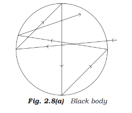
Black body — An ideal body that absorbs and emits radiation of all frequencies uniformly.
Black Bodies and Their Radiation
- Ordinary objects: Usually reflect, absorb and transmit different portions of incident radiation; they are imperfect absorbers.
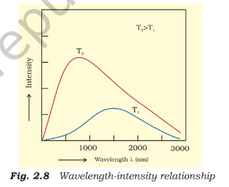
- Ideal behaviour: A black body is a perfect absorber and radiator, and its radiation intensity and spectral distribution depend only on its temperature.
- Thermal equilibrium: In a given time, it emits the same energy per unit area as it absorbs from its surroundings.
- Practical models: Carbon black approximates a black body; a closed cavity with a tiny hole is a good physical model because entering rays undergo repeated reflections and are eventually absorbed.
How Black-Body Emission Changes
- At fixed temperature: Intensity rises with wavelength to a maximum, then falls as wavelength increases further.
- As temperature rises: The peak shifts to shorter wavelengths; the emitted radiation becomes richer in blue light.
- Example: Heated iron glows dull red, then brighter red, then white and, at very high temperatures, blue.
Planck’s Quantum Theory
Planck’s Explanation
- In 1900: Max Planck gave the first successful explanation of black-body radiation.
- Oscillators: He treated atoms in the black-body walls as oscillators that exchange energy with electromagnetic radiation.
- Quantisation: Atoms and molecules emit or absorb energy only in discrete packets, rather than continuously.
- Quantum: The smallest amount of energy emitted or absorbed as electromagnetic radiation.
The energy of a quantum is proportional to its radiation frequency.
Symbols and Permitted Energies
- Symbols: is quantum energy, is frequency, and is Planck’s constant.
- Planck’s constant: .
- Allowed oscillator energies: , where ; intermediate energy values are not allowed.
Staircase Energy
Like standing on staircase steps, an oscillator can have only specific energy levels; it cannot sit between them.
State Planck’s quantum theory and write the energy equation for a quantum.
Quick recap
- Classical physics could not explain several radiation and atomic phenomena, including black-body radiation.
- A black body perfectly absorbs and emits radiation; its spectrum depends only on temperature.
- Increasing temperature shifts the emission maximum toward shorter wavelengths.
- Planck proposed in 1900 that energy exchange occurs in discrete quanta.
- A quantum has energy , and oscillator energies are restricted to .
Photoelectric Effect
Photoelectric Effect and Its Observations
Photoelectric effect — The emission of electrons from a metal surface when light of sufficiently high frequency shines on it.
Key observations
- First observed: H. Hertz observed the effect in 1887 using metals such as potassium, rubidium and caesium.
- Immediate emission: Electrons are emitted as soon as suitable light strikes the metal; there is no time lag.
- Intensity: At a frequency above the threshold, greater light intensity ejects more electrons.
- Threshold frequency: Each metal has a minimum frequency, ; below it, no electrons are emitted, regardless of intensity.
- Frequency and kinetic energy: Above , increasing the light frequency increases the kinetic energy of emitted electrons.
Classical Physics and the Threshold Frequency
Why the observations mattered
- Classical expectation: Light energy was thought to depend on brightness, so both the number and kinetic energy of emitted electrons should rise with intensity.
- Observed result: Intensity affects the number of emitted electrons, but their kinetic energy depends on frequency, not brightness; classical physics could not explain this.
- Potassium example: Red light at – produces no photoelectrons, even at high intensity; weak yellow light at – does.
- Potassium threshold: ; increasing red-light brightness cannot compensate for frequency below this value.
Work function — The minimum energy required to remove an electron from a metal; it is denoted by or .
A metal’s work function equals the energy of a photon at its threshold frequency.
| Metal | Li | Na | K | Mg | Cu | Ag |
|---|---|---|---|---|---|---|
| (eV) |
Einstein’s Photon Explanation
Photon model
- Einstein (1905): Explained the photoelectric effect using Planck’s quantum theory of radiation.
- Photon: Light can be treated as particles, each carrying energy .
- Energy transfer: A photon transfers its energy to an electron in one interaction; if sufficient, the electron is ejected immediately.
- Kinetic energy: The photon’s energy beyond the work function becomes the emitted electron’s kinetic energy.
- Intensity: A more intense beam contains more photons, so it can eject more electrons.
Use frequency or wavelength to calculate the energy of one photon.
Emission occurs when ; at the threshold, the maximum kinetic energy is zero.
Dual Behaviour of Electromagnetic Radiation
Wave-particle duality — Light has both wave-like and particle-like properties; which aspect is observed depends on the experiment.
| Aspect | Wave behaviour | Particle behaviour |
|---|---|---|
| When observed | As light propagates | When radiation interacts with matter |
| Evidence or example | Interference and diffraction | Photoelectric effect and black-body radiation |
- Extension: Microscopic particles such as electrons also exhibit wave-particle duality.
How does light intensity affect photoelectric emission?
State Einstein’s photoelectric equation and define the work function.
A metal has threshold frequency . Find the kinetic energy of an electron emitted by light of frequency .
Quick recap
- Photoelectric emission is immediate and occurs only when the incident frequency reaches the metal’s threshold frequency.
- Above threshold, light intensity controls the number of emitted electrons; frequency controls their maximum kinetic energy.
- The work function is , the minimum energy needed to eject an electron.
- Einstein’s equation is ; photon energy is .
- Light shows particle behaviour when interacting with matter and wave behaviour in interference and diffraction.
- Microscopic particles, including electrons, can also exhibit wave-particle duality.
Evidence for the quantized lectronic Energy Levels: Atomic spectra
Continuous Spectrum
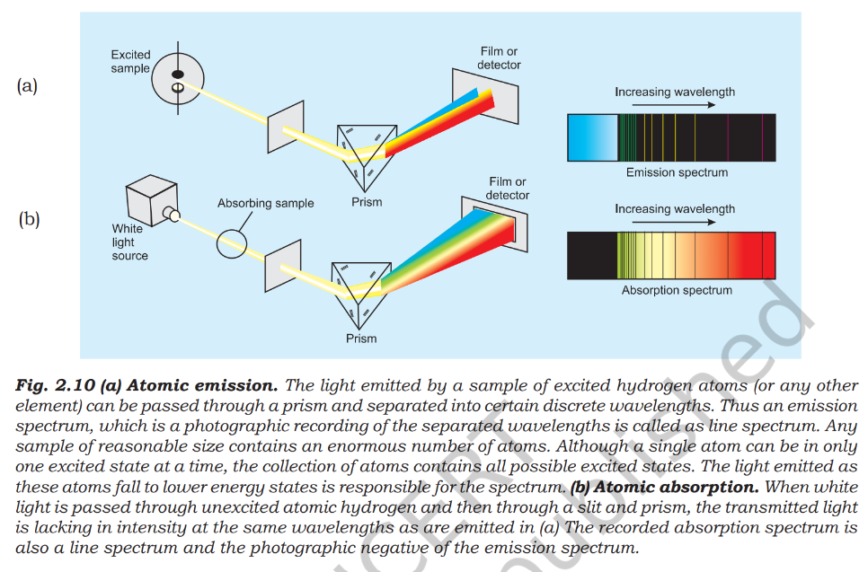
- Continuous spectrum: A spectrum containing an uninterrupted range of wavelengths, with colours merging gradually into one another.
- Example: White light dispersed by a prism forms a continuous spectrum from violet to red.
Emission and Absorption Spectra
Absorption spectrum — The pattern formed when a sample absorbs specific wavelengths from continuous radiation, leaving dark lines or spaces.
| Point | Emission spectrum | Absorption spectrum |
|---|---|---|
| How it forms | Excited matter emits radiation | Matter absorbs selected wavelengths from continuous radiation |
| Appearance | Bright lines on a dark background | Dark lines in a bright continuous spectrum |
Spectroscopy — The study of emission or absorption spectra.
Atomic Line Spectra
- Line spectrum: Gas-phase atoms emit only certain wavelengths, producing separate bright lines with dark spaces rather than a continuous spread.
- Quantized energies: Discrete spectral lines provide evidence that atoms exchange energy only in specific amounts.
- Figure 1: Emission appears as bright lines; absorption appears as dark lines within a continuous spectrum.
Using Line Spectra to Identify Elements
- Unique pattern: Each element has its own characteristic line emission spectrum, like a fingerprint.
- Chemical analysis: Match the emission lines of an unknown sample with those of known elements to identify it.
- Robert Bunsen: Among the early investigators to use line spectra for identifying elements.
- Spectroscopic discoveries: Rubidium, caesium, thallium, indium, gallium and scandium were identified through analysis of minerals; helium was first discovered in the Sun by spectroscopy.
Line Spectrum of Hydrogen
For visible hydrogen lines, ; is wavenumber.
Rydberg Formula and Hydrogen Series
- Rydberg constant: For hydrogen, is the Rydberg constant.
- Allowed integers: and .
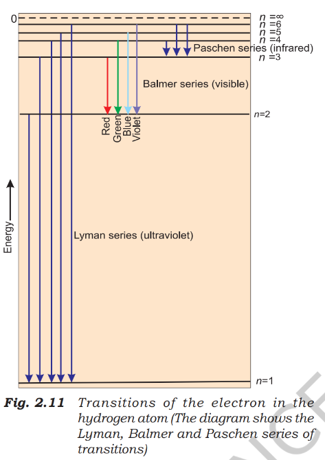
- Series rule: Keep fixed; the emitted lines correspond to transitions from higher levels down to .
This expression describes all hydrogen spectral series.
| Series | Fixed level | Higher levels | Spectral region |
|---|---|---|---|
| Lyman | Ultraviolet | ||
| Balmer | Visible | ||
| Paschen | Infrared | ||
| Brackett | Infrared | ||
| Pfund | Infrared |
Common Features of Atomic Spectra
- Hydrogen: It has the simplest atomic line spectrum; spectra become more complex for heavier atoms.
- Shared features: Each element has a unique line spectrum, and its lines show regularity.
- Importance: These patterns help explain the electronic structure of atoms.
How do emission and absorption spectra differ?
State the Rydberg formula and name the first five hydrogen series.
Quick recap
- A prism separates white light into a continuous spectrum; violet bends more than red.
- Emission produces bright lines; absorption produces dark lines within a continuous spectrum.
- Each element has a unique line spectrum that can identify it.
- Hydrogen's Balmer series is visible and follows the Balmer formula.
- The Rydberg formula describes hydrogen lines; fixed values define spectral series.
- Hydrogen's first five series are Lyman, Balmer, Paschen, Brackett and Pfund.
Bohr’s Model For Hydrogen Atom
Bohr’s Postulates
The frequency of radiation equals the energy difference between the two states divided by Planck’s constant. Here is the lower and the higher energy.
Quantisation of Angular Momentum
Here is electron mass, its speed, the orbit radius, and is a positive integer.
Hydrogen Energy Levels and Orbit Radii
Use for the radius of the hydrogen electron’s th stationary orbit.
. The negative sign indicates a bound electron, with zero energy defined for a free electron infinitely far from the nucleus.
Energy-level examples
- Ground state: At , ; this is the most stable, most tightly bound state.
- Second state: At , , which is higher (less negative) than .
- Ionisation limit: A free electron has and energy .
Hydrogen-like Species
Use these expressions for a one-electron species of nuclear charge ; energy is in joules and radius in picometres.
Electron speed
- Nuclear charge: Electron speed increases as the positive charge on the nucleus increases.
- Orbit level: Electron speed decreases as the principal quantum number increases.
Do not treat negative energy as negative stability: it means the electron’s energy is below the zero-energy reference for a free electron. More negative energy means stronger binding.
What does the negative sign in hydrogen’s energy mean?
How do the energy and radius of a hydrogen-like ion change as increases?
Quick recap
- Bohr’s model allows electrons to occupy only fixed, quantised orbits.
- Angular momentum is quantised: .
- Hydrogen orbit radii follow , where .
- Hydrogen energy levels follow ; is the ground state.
- A free electron at infinity has zero energy; bound electron energies are negative.
- For one-electron ions, increasing makes energy more negative and radius smaller.
Explanation of Line Spectrum of Hydrogen
Hydrogen Line Spectrum and Bohr’s Model
Hydrogen line spectrum — Distinct spectral lines produced when hydrogen electrons absorb or emit photons during transitions between fixed energy levels.
Energy transitions
- Absorption: An electron moves from a lower orbit to a higher orbit and absorbs energy.
- Emission: An electron moves from a higher orbit to a lower orbit and emits energy.
- Spectral lines: Each line corresponds to a particular transition; many hydrogen atoms can undergo different transitions.
- Intensity: The brightness of a line depends on the number of photons with that wavelength or frequency.
- Sign: For emission, is negative; use the magnitude of the emitted energy to calculate photon frequency.
Here, and are the initial and final principal quantum numbers; .
For emitted radiation, use to find the positive frequency.
Wavenumber is frequency divided by the speed of light; the hydrogen coefficient is approximately .
Example: transition from to
- Transition: The electron falls from to , producing an emission line in the visible Balmer series.
- Energy change: .
- Photon frequency: .
- Wavelength: .
For a hydrogen-like ion, is its nuclear charge and is the orbit number.
Use this relation to find the radius of orbit for a hydrogen-like ion.
Example: first orbit of
- Values: For , and the first orbit has .
- Energy: .
- Radius: .
Link with Rydberg’s expression
- Agreement: Bohr’s energy-transition expression has the same form as the Rydberg expression derived empirically from spectral data.
- Meaning: Quantised hydrogen energy levels explain why its spectrum contains distinct lines rather than a continuous range.
Limitations of Bohr’s Model
- Success: It explained the stability and line spectra of hydrogen and hydrogen-like ions such as , and .
- Fine structure: It could not explain the closely spaced doublet lines in the hydrogen spectrum.
- Other atoms: It could not explain spectra of atoms other than hydrogen, including helium.
- External fields: It could not explain spectral-line splitting in a magnetic field (Zeeman effect) or an electric field (Stark effect).
- Chemical bonding: It could not explain how atoms form molecules through chemical bonds.
Why a new atomic model was needed
- Bohr’s model has limitations beyond hydrogen-like atoms.
- A more general theory is needed to explain complex atoms and chemical bonding.
- Two important developments: dual behaviour of matter and the Heisenberg uncertainty principle.
Dual Behaviour of Matter
de Broglie hypothesis — Proposed in 1924, it states that matter, like radiation, has both particle-like and wave-like behaviour.
For a moving particle, is Planck’s constant, is mass, is velocity and is momentum.
Evidence and significance
- Electron diffraction: An electron beam undergoes diffraction, confirming its wave behaviour.
- Electron microscope: It uses electron waves and can achieve magnification of about 15 million times.
- Small particles: Electrons and other subatomic particles have detectable wavelengths because their masses are very small.
- Everyday objects: Moving objects also have wave character, but their large masses make their wavelengths too short to detect.
Examples of de Broglie wavelengths
- Ordinary object: A ball moving at has , far too small to detect.
- Electron: For an electron of mass with kinetic energy , the speed is about and the wavelength is about .
- Photon mass example: For a photon of wavelength , using in gives .
How does Bohr’s model explain the hydrogen line spectrum?
State two limitations of Bohr’s model.
Quick recap
- Electron transitions between fixed hydrogen energy levels produce distinct spectral lines.
- Use ; emission gives a negative energy change, but photon frequency uses its magnitude.
- Each spectral line represents a particular transition; line intensity depends on the number of photons absorbed or emitted.
- Bohr’s model explains hydrogen and hydrogen-like ions but not fine structure, multi-electron spectra, field splitting or bonding.
- For hydrogen-like ions, and .
- The de Broglie relation assigns wave behaviour to moving matter; it is detectable for subatomic particles but not ordinary objects.
Heisenberg’s Uncertainty Principle
Statement and Mathematical Form
Heisenberg’s Uncertainty Principle — It is impossible to determine simultaneously the exact position and exact momentum (or velocity) of a particle such as an electron.
- Origin: Werner Heisenberg stated the principle in 1927; it follows from the dual behaviour of matter and radiation.
- Trade-off: Greater precision in position means greater uncertainty in velocity, and vice versa.
- Measurement: Measurements of an electron’s position or velocity therefore give a fuzzy, not perfectly precise, description.
Here, is uncertainty in position, is uncertainty in momentum, is mass, and is uncertainty in velocity.
Why Measurement Affects an Electron
- Resolution: Locating an electron accurately requires radiation with a wavelength smaller than the scale being measured.
- Photon momentum: Such short-wavelength photons have high momentum, given by .
- Disturbance: A photon can collide with the electron and change its momentum. Its position may be located, but its velocity after the collision becomes uncertain.
- Analogy: Measuring paper thickness with an unmarked metre stick is inaccurate; a suitable instrument needs finer graduations. An electron requires an extremely fine scale, which itself involves energetic photons.
Significance: No Definite Electron Trajectory
- Trajectory: A trajectory is a definite path described by an object’s positions and velocities at different times.
- Classical prediction: Knowing an object’s position, velocity and acting forces allows its later position to be predicted.
- For electrons: Position and velocity cannot both be known with arbitrary precision at the same instant; therefore, an electron cannot be assigned a definite path or trajectory.
- Quantum description: Exact path descriptions are replaced by probabilities of finding an electron at a given position and with a given momentum.
Effect on Macroscopic and Microscopic Objects
| Point | Macroscopic objects | Microscopic objects |
|---|---|---|
| Uncertainty effect | Negligible for milligram-sized or heavier objects. | Significant for particles such as electrons. |
| Illustrative value of | For a mass of , it is about . | For an electron, it is about . |
| Consequence | Does not meaningfully limit measurement precision. | Makes precise classical paths unsuitable. |
The minimum product decreases as mass increases. Using gives the approximate examples above.
Electron example
- Electron mass: gives an uncertainty product of approximately .
- If position is known to , then .
- Meaning: This large velocity uncertainty rules out the classical picture of an electron moving in a fixed Bohr orbit.
An electron is located within . What is the uncertainty in its velocity?
A golf ball of mass moves at . If its speed is measured to accuracy, find the uncertainty in position.
Why the Bohr Model Fails
From Bohr’s fixed orbits to the quantum model
- Bohr model treats the electron as a charged particle in a well-defined circular orbit.
- A definite orbit requires exact position and velocity at the same time.
- The uncertainty principle makes this simultaneous precision impossible; the model also neglects the electron’s wave character.
- Therefore, fixed electron orbits are inconsistent with wave–particle duality and the uncertainty principle.
- Quantum mechanics replaces fixed paths with a description consistent with duality and probability.
Why can an electron not be said to move in a definite Bohr orbit?
Quick recap
- The uncertainty principle, stated by Heisenberg in 1927, limits simultaneous precision in an electron’s position and momentum.
- The product of position and momentum uncertainties is at least .
- More accurate position knowledge means greater uncertainty in velocity, and vice versa.
- Uncertainty has meaningful effects for electrons but negligible effects for macroscopic objects.
- Electrons cannot be assigned definite trajectories; quantum mechanics describes their likely positions instead.
- The Bohr model’s fixed orbits conflict with the uncertainty principle and neglect wave–particle duality.
Quantum Mechanical Model Of Atom
Quantum Mechanics
Quantum mechanics — The branch of science that describes microscopic objects by accounting for their wave-like and particle-like behaviour.
- Classical mechanics describes macroscopic objects well, but does not adequately explain microscopic particles such as electrons.
- Reason for failure: Classical mechanics does not account for matter’s dual behaviour or the uncertainty principle.
- Macroscopic limit: When wave-like effects are insignificant, quantum mechanics gives results equivalent to classical mechanics.
- Development: Werner Heisenberg and Erwin Schrödinger independently developed quantum mechanics in 1926.
| Feature | Classical mechanics | Quantum mechanics |
|---|---|---|
| Best suited to | Macroscopic objects | Microscopic objects |
| Behaviour considered | Primarily particle-like | Both wave-like and particle-like |
| Macroscopic limit | Describes motion directly | Agrees with classical results when wave effects are insignificant |
Schrödinger Equation
- Schrödinger equation: For a system whose energy does not change with time, it relates the system’s energy to its wave function.
- Hamiltonian (): A mathematical operator constructed from the system’s total-energy expression.
- Total energy: Includes kinetic energies of the subatomic particles and attractive or repulsive potential interactions among them.
- Solution: Solving the equation gives the allowed energy, , and wave function, .
- Wave-particle link: Schrödinger’s equation incorporates de Broglie’s wave-particle duality; solving it generally requires advanced mathematics.
- 1926Heisenberg and Schrödinger independently developed quantum mechanics.
- 1933Schrödinger received the Nobel Prize in Physics.
Hydrogen Atom and Atomic Orbitals
- Hydrogen solutions: Solving Schrödinger’s equation gives the electron’s allowed energy levels and corresponding wave functions.
- Quantum numbers: Each hydrogen energy state and wave function is characterized by three quantum numbers: principal quantum number , azimuthal quantum number , and magnetic quantum number .
- Wave function (): A mathematical function that depends on the electron’s coordinates; by itself, it has no direct physical meaning.
- Atomic orbital: The wave function for an electron in an atom; it describes an allowed electron state and has a definite energy.
- One-electron systems: Hydrogen and hydrogen-like species have one electron; their wave functions are called atomic orbitals.
The probability of finding an electron at a point is proportional to the probability density there.
- Probability density: is always positive; its values across space show where the electron is most likely to be found.
- Hydrogen spectrum: Quantum-mechanical calculations predict the hydrogen spectrum, including features the Bohr model could not explain.
Multi-electron Atoms
- Exact solutions: Schrödinger’s equation cannot be solved exactly for multi-electron atoms, so approximate methods are used.
- Orbital shapes: Computer calculations show that these atoms’ orbitals are not radically different from hydrogen orbitals.
- Nuclear charge: The greater nuclear charge makes multi-electron orbitals somewhat contracted.
- Energy dependence: In hydrogen-like species, orbital energies depend only on ; in multi-electron atoms, they depend on both and .
Key Features of the Quantum Mechanical Model
- Quantized energy: Electrons bound in atoms can have only certain specific energy values; these allowed solutions arise from their wave-like properties.
- Uncertainty principle: An electron’s exact position and exact velocity cannot be determined simultaneously, so its path cannot be known accurately.
- Atomic orbital: An orbital is an electron’s wave function; an atom can have many possible orbitals, each with a definite energy.
- Orbital capacity: An orbital can contain no more than two electrons.
- Filling order: In a multi-electron atom, electrons occupy orbitals in order of increasing energy.
- Electron information: The orbital wave function contains the information used to describe an electron in an atom.
Why is the path of an electron in an atom not known accurately?
Quick recap
- Quantum mechanics describes microscopic objects through wave-like and particle-like behaviour.
- For a system with constant energy, Schrödinger’s equation is ; its solutions give and .
- Hydrogen solutions are characterized by the principal quantum number , azimuthal quantum number , and magnetic quantum number .
- An atomic orbital is an electron’s wave function; the probability density indicates where it is most likely to be found.
- Exact electron position and velocity cannot be known simultaneously, so an electron’s path is not accurately determined.
- An orbital holds at most two electrons; multi-electron atoms fill orbitals in increasing energy order.
- Hydrogen-like orbital energies depend on , while multi-electron orbital energies depend on and .
Orbitals and Quantum Numbers
Orbitals and their identification
Atomic orbital — A quantum-mechanical one-electron wave function that describes an electron’s probable distribution in an atom.
- Distinguishing features: Orbitals differ in size, shape and orientation, which indicate where an electron is more likely to be found.
- Quantum numbers: The three quantum numbers , and identify an orbital.
Principal quantum number, n
Principal quantum number, — A positive integer that identifies the shell and indicates an orbital’s size and, to a large extent, its energy.
- Allowed values: ; each value identifies a shell.
- Shell names: correspond to the K, L, M and N shells.
- Size and energy: Increasing generally means a larger orbital and higher energy; the electron is, on average, farther from the nucleus.
- Hydrogen-like species: For hydrogen, and , orbital size and energy depend only on .
The total number of orbitals in a shell is the square of its principal quantum number.
Azimuthal quantum number, l
Azimuthal quantum number, — The quantum number that identifies a subshell and determines the three-dimensional shape of an orbital; it is also called the orbital angular momentum or subsidiary quantum number.
For a given shell, there are possible values of , starting at zero.
| Subshell | Number of orbitals | |
|---|---|---|
- Subshell count: The shell with principal quantum number contains subshells.
- Examples: has ; has ; and has .
- Energy in multi-electron atoms: The value of also influences orbital energy.
Magnetic orbital quantum number, ml
Magnetic orbital quantum number, — The quantum number that specifies an orbital’s spatial orientation within a subshell.
For each value of , there are possible values of and therefore orbitals in the subshell.
| Subshell | Allowed | Number of orbitals | |
|---|---|---|---|
- Dependence: Allowed values of come from , and allowed values of come from .
- Orbital identification: , , identifies one orbital in the subshell.
Electron spin quantum number, ms
Electron spin quantum number, — The fourth quantum number, which describes one of the two possible orientations of an electron’s intrinsic spin.
- Why introduced: In 1925, George Uhlenbeck and Samuel Goudsmit proposed electron spin to help explain closely spaced doublets and triplets in multi-electron spectra.
- Spin values: or ; these are represented by spin-up and spin-down .
- Opposite spins: Two electrons with different values have opposite spins.
- Orbital capacity: An orbital holds at most two electrons, and they must have opposite spins.
| Quantum number | Identifies or describes |
|---|---|
| Shell; orbital size and, to a large extent, energy | |
| Subshell; orbital shape | |
| Orbital orientation | |
| Electron spin orientation |
Orbit, orbital and probability
| Point | Orbit | Orbital |
|---|---|---|
| Meaning | Bohr’s proposed circular path of an electron around the nucleus | Quantum-mechanical one-electron wave function, |
| Description | A definite path; the exact path cannot be established according to the Heisenberg uncertainty principle | Described by , and ; its value depends on the electron’s coordinates |
| Physical significance | A definite Bohr path has no real physical meaning and cannot be demonstrated experimentally | itself has no physical meaning; gives probability density |
Probability density
- Probability density: gives the probability per unit volume at a point in the atom.
- Probability in a small volume: The probability of finding the electron in a small volume element is approximately multiplied by that volume.
- Probability in a region: Add the probability contributions from the small volume elements throughout the region to obtain the total probability.
How many orbitals are associated with the shell ?
Name the subshells for , , and .
How do orbit and orbital differ?
Quick recap
- The three quantum numbers , and identify an orbital.
- identifies the shell; the total number of orbitals in a shell is .
- identifies the subshell and shape; its values range from to .
- specifies orbital orientation and has possible values.
- describes spin orientation and can be or ; two electrons in one orbital have opposite spins.
- An orbital is not a definite path; is the probability density.
Shapes of Atomic Orbitals
Wavefunctions, Probability Density and Nodes
Orbital wavefunction — The wavefunction is a mathematical function of an electron’s coordinates; by itself, it has no direct physical meaning.
Probability density
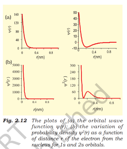
- Born interpretation: The probability density at a point is given by ; a higher value means a greater likelihood of finding the electron there.
- orbital: Probability density is greatest at the nucleus and decreases sharply with distance.
- orbital: Probability density falls to zero at a node, rises to a small maximum, and then approaches zero farther from the nucleus.
- Node: A region or surface where probability density is zero; for orbitals, the number of nodes is .
Boundary Surfaces and s Orbitals
Boundary-surface diagrams
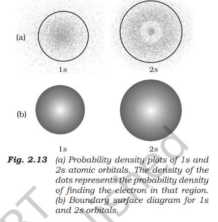
- Boundary surface: A surface enclosing a region where the probability density is constant; it represents an orbital’s shape.
- Useful boundary: The diagram is usually drawn to enclose a region with about probability of finding the electron.
- Not : Probability density remains non-zero, however small, at every finite distance from the nucleus, so no finite boundary encloses the electron with certainty.
- Charge-cloud view: In a dot diagram, denser dots indicate regions of greater electron probability.
s orbitals
- Shape: Every orbital is spherical and spherically symmetric; probability at a fixed distance from the nucleus is equal in every direction.
- Size: Orbital size increases with principal quantum number ; the order is .
- Position: As increases, the electron is generally found farther from the nucleus.
p Orbitals
Shape, orientation and size
- Shape: Each orbital has two lobes on opposite sides of a plane through the nucleus; probability density is zero on that plane.
- Three orientations: The orbitals are labelled , and ; their axes are mutually perpendicular.
- Quantum number: For , the three possible values correspond to three orbitals, but do not map directly to the , and directions.
- Same properties: The three orbitals in a subshell have identical size, shape and energy; they differ in orientation.
- Size and energy: Both increase with ; for the listed orbitals, the order is .
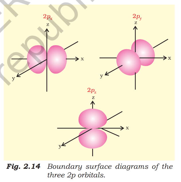
Nodes in p orbitals
- Radial nodes: In a orbital, the number is ; for example, has one and has two.
- Angular node example: The -plane is a nodal plane for the orbital.
d Orbitals and General Node Counts
d orbitals
- Quantum numbers: For a orbital, ; since , the minimum principal quantum number is .
- Number of orbitals: The five possible values, , give five orbitals.
- Names: The five orbitals are , , , and .
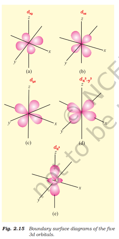
Angular and total nodes
- Angular nodes: These are nodal planes through the nucleus; their number equals .
- Examples: A orbital has one angular node and a orbital has two; has the - and -planes as nodal planes.
- Total nodes: The total is the sum of radial and angular nodes, and equals .
Use these relations for an orbital with principal quantum number and azimuthal quantum number .
Do not confuse orbital shape with a sharp electron boundary: a boundary-surface diagram encloses a high-probability region, usually about , not a region of certainty.
What is a node, and how many total nodes does an orbital have?
How do the shapes of s and p orbitals differ?
Quick recap
- The wavefunction is mathematical; gives probability density.
- A node is where probability density is zero; total nodes equal .
- Boundary-surface diagrams usually enclose about probability, not .
- All orbitals are spherical; their size increases with .
- There are three mutually perpendicular orbitals, each with two lobes.
- For orbitals, and there are five orbitals; angular-node count equals .
Energies of Orbitals
Orbital Energies in Hydrogen and Multi-Electron Atoms
Hydrogen atom
- Energy depends only on : In a hydrogen atom, orbitals with the same principal quantum number have equal energy, even if their shapes differ.
- Degenerate orbitals: Orbitals with equal energy are called degenerate; for example, and are degenerate in hydrogen.
- Energy order: .
- Ground state: An electron in is in the lowest-energy, most stable state and is most strongly held by the nucleus.
- Excited state: An electron in , , or any higher orbital is in an excited state.
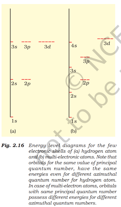
Orbital Energies in Multi-Electron Atoms
Shielding, penetration and energy splitting
- Shielding: Within the same shell, electrons shield outer electrons more effectively than electrons; electrons shield more effectively than electrons.
- Penetration: An electron spends more time close to the nucleus than a electron, which in turn penetrates more than a electron.
- Effective nuclear charge: For a given shell, the effective nuclear charge experienced by an electron decreases as the azimuthal quantum number increases.
- Energy within a shell: Greater penetration means stronger attraction to the nucleus and lower energy: .
- Energy splitting: Different shielding and penetration give subshells in the same shell different energies in multi-electron atoms. Their energies depend on both and , unlike in hydrogen.
A simple rule for comparing orbital energies in multi-electron atoms.
Applying the energy rule
- Lower sum: The orbital with the smaller value of has lower energy.
- Tie-breaker: If two orbitals have the same , the orbital with the smaller has lower energy.
- Example: and both have ; because for is smaller, has lower energy than .
- Energy order: Applying the rule gives .
| Orbital | Energy comparison | |||
|---|---|---|---|---|
| 1 | 0 | 1 | Lowest among these orbitals | |
| 2 | 0 | 2 | Lower than | |
| 2 | 1 | 3 | Lower than ; same sum, smaller | |
| 3 | 0 | 3 | Higher than | |
| 3 | 1 | 4 | Lower than | |
| 4 | 0 | 4 | Higher than | |
| 3 | 2 | 5 | Lower than | |
| 4 | 1 | 5 | Higher than |
Effect of increasing nuclear charge
- Within the same subshell: Orbital energy decreases as the effective nuclear charge increases.
- Example: The orbital energy decreases in the order .
State the rule for comparing orbital energies.
Why do subshells of the same shell have different energies in multi-electron atoms?
Quick recap
- In hydrogen, orbital energy depends only on ; orbitals with the same are degenerate.
- The orbital is the ground state; electrons in higher orbitals are in excited states.
- In multi-electron atoms, subshell energies depend on both and because shielding and penetration differ.
- Within a shell, penetration is greatest for , then , then ; energy increases in the order .
- The rule compares orbital energies; when sums are equal, the orbital with smaller has lower energy.
- Within the same subshell, energy decreases as increases.
Filling of Orbitals in Atom
Aufbau Principle
Aufbau principle — In the ground state, electrons occupy available orbitals in order of increasing energy, filling lower-energy orbitals before higher-energy ones.
Orbital filling order
- Usual order: .
- Energy dependence: Orbital energies depend on effective nuclear charge; therefore, there is no single ordering that is exact for every atom.
- Useful guide: The order is a practical guide, especially for placing outermost valence electrons; exceptions occur when orbitals have similar energies.
- Example: Potassium’s valence electron occupies rather than according to this order.
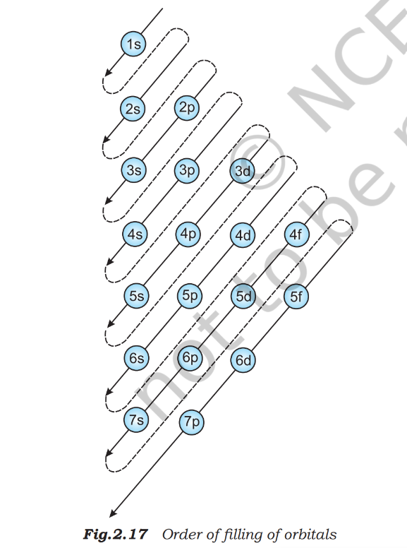
Pauli Exclusion Principle
Pauli exclusion principle — No two electrons in an atom can have the same set of four quantum numbers.
Consequences and capacity
- One orbital: Holds at most two electrons, and they must have opposite spins.
- Quantum numbers: Two electrons in the same orbital share , and , but have opposite spin quantum numbers.
- Attribution: The principle was given by Wolfgang Pauli in 1926.
| Subshell | Number of orbitals | Maximum electrons |
|---|---|---|
For a shell with principal quantum number .
Hund’s Rule of Maximum Multiplicity
Hund’s rule of maximum multiplicity — In a set of degenerate orbitals, electrons occupy each orbital singly before any pairing begins.
Applying Hund’s rule
- Degenerate orbitals: Orbitals in the same subshell (, or ) have equal energy.
- Filling pattern: Each orbital receives one electron before electrons begin to pair.
- Pairing begins: In , and subshells, pairing starts with the 4th, 6th and 8th electron, respectively.
- Stability: Half-filled and fully filled degenerate sets gain extra stability due to their symmetry.
State the Aufbau principle and give the usual initial orbital filling order.
How many electrons can a shell with principal quantum number hold at most?
State Hund’s rule and explain when pairing begins in a subshell.
Quick recap
- Electrons generally fill orbitals from lower to higher energy (Aufbau principle).
- The filling sequence is a useful guide, but close orbital energies can cause exceptions.
- An orbital holds at most two electrons with opposite spins (Pauli exclusion principle).
- A shell with principal quantum number holds at most electrons.
- Degenerate orbitals fill singly before pairing (Hund’s rule).
- Half-filled and fully filled degenerate sets have extra stability due to symmetry.
Electronic Configuration of Atoms
Meaning and representations

Filling orbitals and writing configurations
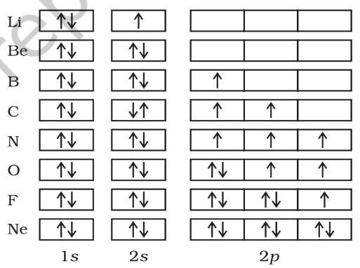
Subshell filling pattern
- Order: The filling sequence begins .
- Later filling: It continues through and , then and ; small energy differences can lead to exceptions.
- Period 3: Sodium to argon fill and then , following the same pattern as lithium to neon.
- Period 4: Potassium and calcium fill before the subshell begins filling at scandium.
- Further pattern: Rubidium to xenon fill ; caesium and barium fill , followed by filling involving and .
- Heavier elements: Filling proceeds through , , and then and . Elements after uranium are short-lived and artificially produced.
Core electrons and shorthand notation
- Core electrons: Electrons in completely filled inner shells.
- Valence electrons: Electrons in the outermost occupied shell; they largely determine an element’s chemical behaviour.
- Shorthand notation: Replace the inner-shell configuration with the symbol of the preceding noble gas in square brackets, then write the remaining electrons; for example, sodium is .
Stable half-filled and completely filled subshells
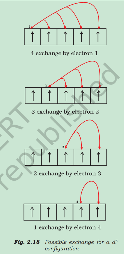
Why electronic configuration matters
- Chemical behaviour: Electron distribution helps explain bonding, why elements are metals or non-metals, and differences in reactivity.
- Examples: Filled outer shells make helium and argon relatively unreactive, while halogens are reactive because their outer shells are not complete.
- Importance: Electronic structure is central to modern explanations of chemical properties.
Do not assume every atom follows a perfectly regular filling pattern: chromium and copper are key exceptions because the more stable and arrangements form.
What is the difference between core and valence electrons?
Why do chromium and copper have exceptional configurations?
Quick recap
- Electronic configuration describes how electrons are distributed among an atom’s orbitals.
- Subshell notation gives electron counts; orbital diagrams show individual orbital occupancy and spins, representing all four quantum numbers.
- Orbitals hold two electrons each; subshell capacities are , , and .
- Electrons fill lower-energy orbitals first; equal-energy orbitals fill singly with parallel spins before pairing.
- Core electrons occupy filled inner shells, while valence electrons are in the shell with the highest principal quantum number.
- Half-filled and filled subshells gain extra stability, explaining exceptions such as Cr and Cu.
Summary
Atoms and Subatomic Particles
Atom — The smallest part of an element that takes part in chemical reactions.
Atomic theory and subatomic particles
- Dalton’s view: In 1808, John Dalton described the atom as the ultimate indivisible particle of matter.
- Experimental evidence: By the end of the nineteenth century, atoms were shown to be divisible and composed of electrons, protons and neutrons.
- Impact: Discoveries of subatomic particles led to atomic models explaining the structure of atoms.
Development of Atomic Models
- 1808John Dalton proposed an atomic theory treating atoms as indivisible.
- 1898J. J. Thomson proposed the embedded-electron model of the atom.
- 1909Rutherford’s alpha-particle scattering experiment challenged Thomson’s model.
- 1913Niels Bohr proposed his model of the hydrogen atom.
- 1926Erwin Schrödinger proposed an equation describing electron distributions and allowed energies.
Thomson and Rutherford Models
| Point | Thomson model | Rutherford model |
|---|---|---|
| Structure | A uniform sphere of positive electricity with electrons embedded in it. | A tiny, positively charged nucleus at the centre, with electrons revolving around it. |
| Evidence and limitation | Rutherford’s alpha-particle scattering experiment showed this model was wrong. | Improved on Thomson’s model, but could not explain atomic stability or electron distribution and relative energies. |
Bohr Model
Postulates and scope
- Allowed orbits: Electrons move around the nucleus in circular orbits, but only certain orbits are permitted.
- Quantized energy: Each allowed orbit has a specific energy; Bohr calculated the electron’s energy and distance from the nucleus for each orbit.
- Success: The model satisfactorily explained the spectrum of hydrogen.
- Limitation: It could not explain spectra of atoms with more than one electron.
- Underlying problem: Treating an electron as a particle moving on a definite circular path ignores its wave character and conflicts with the Heisenberg uncertainty principle.
Heisenberg uncertainty principle — The exact position and exact velocity of an electron cannot both be known at the same time; therefore, its path cannot be completely specified.
Quantum-Mechanical Model
Schrödinger equation and hydrogen atom
- Schrödinger equation: Proposed in 1926 to describe electron distributions in space and the allowed energy levels in atoms.
- Basis: It incorporates de Broglie’s wave-particle duality and is consistent with the Heisenberg uncertainty principle.
- Solutions for hydrogen: Give the possible electron energy states and an associated wave function, , for each state.
- Quantum numbers: Each state is characterized by the principal quantum number , azimuthal quantum number and magnetic quantum number .
- Restrictions: The allowed values of these quantum numbers arise naturally from solving the equation.
- Success: The model explains all aspects of the hydrogen spectrum, including phenomena that Bohr’s model could not explain.
Electron organisation
- The atom’s electron distribution is divided into shells.
- Each shell contains one or more subshells.
- Each subshell contains one or more orbitals, which electrons occupy.
| System | Energy pattern |
|---|---|
| Hydrogen and hydrogen-like ions | All orbitals within the same shell have the same energy; examples include and . |
| Multi-electron atoms | Orbital energy depends on both and . |
Orbital filling and electron configuration
- Energy order: In multi-electron atoms, an orbital with lower has lower energy.
- Tie-break rule: If two orbitals have the same , the one with lower has lower energy.
- Filling: Electrons occupy orbitals in order of increasing energy, following the Pauli exclusion principle and Hund’s rule.
Pauli exclusion principle — No two electrons in an atom can have the same set of four quantum numbers.
Hund’s rule of maximum multiplicity — Within a subshell, electrons occupy each orbital singly before any pairing takes place.
Do not confuse a Bohr orbit (a definite path) with a quantum-mechanical orbital (a state occupied by electrons).
Quick recap
- Atoms are divisible and contain electrons, protons and neutrons.
- Rutherford’s model introduced the small positive nucleus but did not explain stability or electron energies.
- Bohr proposed allowed, quantized orbits; his model explains hydrogen’s spectrum but not multi-electron spectra.
- The Schrödinger model incorporates wave-particle duality and the uncertainty principle, describing allowed states using quantum numbers.
- Electrons occupy orbitals within subshells and shells; multi-electron orbital energies follow the rule.
- Orbital filling follows the Pauli exclusion principle and Hund’s rule.
Chemistry — ALL CHAPTERS
1
Some Basic Concepts Of Chemistry
2
Structure Of Atom
3
Classification Of Elements And Periodicity In Properties
4
Chemical Bonding And Molecular Structure
5
Thermodynamics
6
Equilibrium
7
Redox Reactions
8
Organic Chemistry – Some Basic Principles And Techniques
9
Hydrocarbons