Class 12 Commerce . Accountancy . Computerised Accounting System . Graphs and Charts for Business Data
Chapter 4: Graphs And Charts For Business Data
Ch 4
Accountancy
Class 12 Commerce
Introduction & Graphs And Charts
Graph — A graph is a pictorial representation of data that shows a relationship between at least two dimensions.
Why use graphs and charts?
- Purpose: Convert accounting data into a visual form that is easier to understand and communicate than raw data.
- Use: Graphs and charts help present business information clearly.
Types of Graphs and Charts
Key features and uses
- Axes: A graph has at least two axes: the -axis is usually horizontal and the -axis is vertical.
- Line graph: May be a single-line graph or a multiple-line graph.
- Multiple-line graph: Different line styles and shades of colour can distinguish the data series and improve clarity.
- Pie chart: Represents multiple sub-groups of a single variable.
- Bar diagram: Depicts two or more variables.
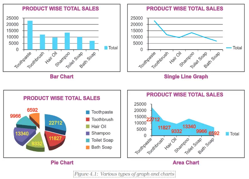
Charts in Excel
- Excel tools: Excel provides standard chart commands on the Ribbon for making different types of graphs and charts.
- Basic approach: Select the worksheet data, open the Insert tab, then choose the desired chart type.
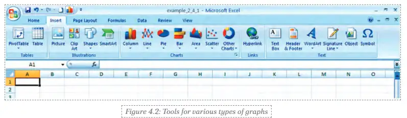
Creating a chart in Excel 2007
- Open the worksheet containing the data.
- Click the Insert tab on the Ribbon.
- Choose the desired chart type to display the data.
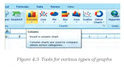
Quick recap
- Graphs and charts present accounting data visually for clearer understanding and communication.
- A graph shows a relationship across at least two dimensions and has at least two axes.
- The -axis is usually horizontal; the -axis is usually vertical.
- Line graphs can be single-line or multiple-line; styles and colours help distinguish series.
- Pie charts show sub-groups of one variable; bar diagrams depict two or more variables.
- In Excel 2007, use the Insert tab to select a chart type for worksheet data.
Basics Steps For Graphs /Charts/ Diagrams Using Excel Part- I
Entering and Organising the Data
Chart or graph — A chart or graph is a pictorial presentation of data that makes comparisons and patterns easier to understand.
Step 1: Enter the worksheet data
- Enter sales for each product across Qtr1–Qtr4, then include product totals and quarter totals.
- Row totals show each product’s total sales; the Total row gives sales by quarter.
- Grand total is the overall sales value, shown where the total row and total column meet.
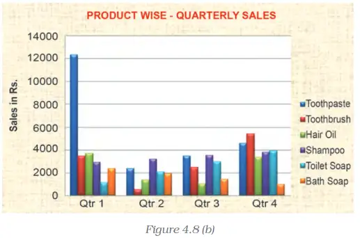
| Product | Qtr1 | Qtr2 | Qtr3 | Qtr4 | Total |
|---|---|---|---|---|---|
| Toothpaste | 12,344 | 2,345 | 3,456 | 4,567 | 22,712 |
| Toothbrush | 3,456 | 500 | 2,456 | 5,415 | 11,827 |
| Hair Oil | 3,678 | 1,345 | 988 | 3,321 | 9,332 |
| Shampoo | 2,900 | 3,190 | 3,480 | 3,770 | 13,340 |
| Toilet Soap | 1,122 | 2,035 | 2,948 | 3,861 | 9,966 |
| Bath Soap | 2,344 | 1,880 | 1,416 | 952 | 6,592 |
| Total | 25,844 | 11,295 | 14,744 | 21,886 | 73,769 |
Creating Charts in Excel
Basic chart-creation process
- Select the data to be charted, including its category labels and values.
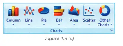
- Open the Insert tab and choose a chart type from the Charts group on the Ribbon.
- Choose a suitable chart or subtype to display the selected data.
- Add or format chart elements as needed.
How can the product-wise sales totals be displayed as a bar chart?
- To chart product-wise total sales, select each product name and its Total value from the worksheet.
- Use Insert > Charts and choose a bar chart.
- The chart compares the six products; Toothpaste has the highest total at Rs. 22,712 thousand.
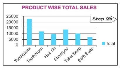
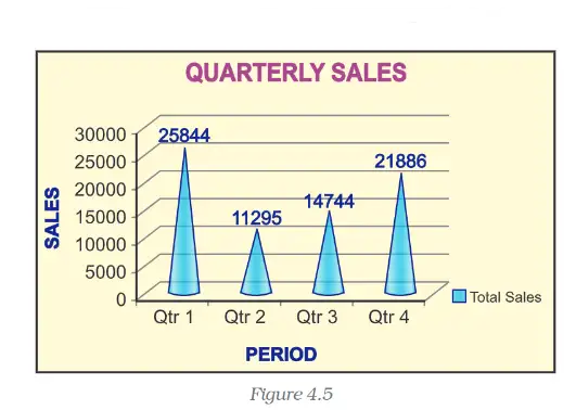
Step 2b: Chart quarter-wise total sales
- Reorganise the worksheet data so the four quarter names and their total sales are together.
- Select the quarter labels and values, then insert a suitable chart from the Ribbon.
- Choose chart types and subtypes to suit the comparison; examples include a column chart, a stacked column chart, a pie chart, or a pie chart in 3-D.
- Combine more than one chart type in a combination chart when the data and comparison require it.
| Period | Total Sales |
|---|---|
| Qtr1 | 25,844 |
| Qtr2 | 11,295 |
| Qtr3 | 14,744 |
| Qtr4 | 21,886 |
| Total | 73,769 |
Elements of a Chart or Graph
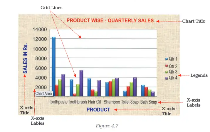
| Element | Meaning |
|---|---|
| Chart area | The entire chart, including all its elements. |
| Plot area | The region where data is plotted; in 2-D it is bounded by the X- and Y-axes, and in 3-D by the X-, Y- and Z-axes. |
| Data point / marker | An individual value shown as a bar, column, line, pie slice or another shape. |
| Data series | Related data points, usually shown in the same colour or pattern. |
| Category (horizontal) axis | Usually the X-axis; displays categories or independent values. |
| Value (vertical) axis | Usually the Y-axis; displays the dependent data values. |
| Legend | Identifies the data series or categories represented by colours or patterns. |
| Chart and axis titles | Descriptive text naming the chart and its axes. |
| Data label | Extra information attached to a data marker, identifying its value or details. |
Displaying and formatting elements
- Default display: Some chart elements appear automatically; others can be added when required.
- Formatting: Elements and the overall chart display can be changed to suit the purpose.
What data should be selected to chart the total sales of each product?
Which quarter had the lowest total sales, and what data would you select to chart quarter-wise sales?
Which chart element identifies the colours or patterns used for different data series?
Quick recap
- Enter the data with product totals, quarter totals and the overall total before charting.
- Select the relevant labels and values, then use Insert > Charts on the Ribbon.
- A bar chart can compare product-wise totals; reorganised data can show quarterly totals.
- Excel offers chart types and subtypes, including stacked column and pie-in-3-D charts, and can combine different chart types.
- Chart area is the whole chart; plot area is where the data is plotted.
- Axes, data markers, series, legends, titles and data labels help explain a chart.
Basics Steps For Graphs /Charts/ Diagrams Using Excel Part- Il
Formatting a Chart with the Design Tab
Selecting and Formatting a Chart Element

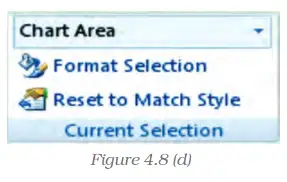
Changing Shape Style, Fill and Effects
- Shape styles: Apply a predefined style or choose a custom fill for the selected chart element.
- Fill and effects: Use colours, pictures, gradients or textures; effects such as bevel, reflection and shadow can enhance its appearance.
Changing Shape Outline
- Outline colour: Choose a theme or standard colour, select a custom colour, or remove the outline with No Outline.
- Line weight: Change the thickness of a line or border using the Weight option.
- Line style: Use Dashes to select a broken-line pattern, or choose further styles under More Lines.
- Arrows: Add an arrow style to a line; additional options are available under More Arrows.
Quick recap
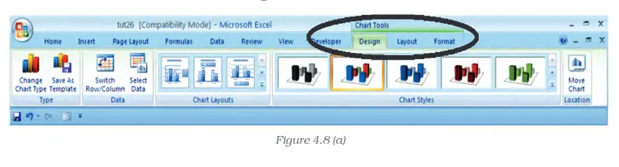
- Click a chart to display the Chart Tools tabs: Design, Layout and Format.
- Use Design options to change chart type, layout and style; Switch Row/Column changes the category and series orientation.
- Select an element directly or from the Chart Elements box, then use Format Selection to edit it.
- Shape Fill includes colours, no fill, picture, gradient and texture options.
- Shape Outline controls colour, visibility, line weight, dashes and arrows.
- Shape Effects include presets, reflection and bevel, when available for the selected element.
Basics Steps For Graphs /Charts/ Diagrams Using Excel Part- Ill
Formatting Chart Text
Chart text formatting — Chart text formatting changes the appearance of text in titles, labels and other chart elements.
- Select the chart element containing the text to format.
- Regular formatting is available from the Mini toolbar or the Font group on the Home tab.
- WordArt formatting is available in the WordArt Styles group on the Format tab.
- Text effects include Text Fill, Text Outline, Shadow, 3-D Format, 3-D Rotation and Text Box.
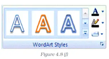
Select a Chart Element from the Ribbon
- Click anywhere in the chart to display the Chart Tools tabs.
- On the Format tab, open the Chart Elements list in the Current Selection group and choose an element.
- Choose the required formatting option from the WordArt Styles group.
Changing the Layout of Chart Elements
Chart layout — Chart layout controls the placement and appearance of chart elements such as labels, axes and backgrounds.
- Layout tab tools can insert or adjust pictures, clip art, data labels and gridlines.
- Format Element dialog lets you choose a category and set options for the selected chart element.

Changing the Chart Type
Changing chart type — A chart type can be changed to present the same data in a form better suited to its purpose.
- Pie chart use is appropriate for showing how categories make up a whole.
- Suitable data for the conversion described consists of one data series with positive, non-zero values.
- Category limit in the Excel version described is seven categories; the categories represent parts of the whole.
- Pie interpretation: each slice represents its category's share, and all slices together represent the total.
Use this to calculate the percentage represented by a category; is its value and is the total.
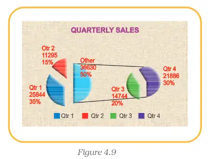
Create and Format a 3-D Pie Chart
- Enter category names and values in two adjacent columns, then select both columns.
- Choose Pie from the chart types on the ribbon, then select 3-D Pie.
- Use the Design tab to choose a chart layout and style.
- On the Format tab, use Shape Effects to apply bevels; set the top and bottom bevel sizes and choose a material if required.
- Use Shape Effects to choose an outer, inner or perspective shadow.
- To change slice orientation, select the plot area and open Format Selection; set the angle of the first slice to a value from 0 to 360 degrees.
- To change workbook theme colours, choose a built-in theme from the Themes group on the Page Layout tab.
Treat the one-series, positive, non-zero data conditions as suitability guidance for the conversion described, not as universal prohibitions for every Excel pie chart or version.
What data is suitable for the pie-chart conversion described?
How can the first slice of a pie chart be rotated?
Quick recap
- Chart text can be formatted with standard font controls or WordArt effects.
- Chart elements can be selected from the Chart Elements list and formatted through ribbon tabs or the Format Element dialog.
- Pie charts show category proportions as slices of one whole.
- Suitable conversion data in the described method has one series of positive, non-zero values; the source notes a seven-category limit for the Excel version described.
- 3-D pie formatting can include layout and style choices, bevels, materials, shadows and rotation.
- Themes change the workbook colours applied to the chart.
Basics Steps For Graphs /Charts/ Diagrams Using Excel Part- IV
Resizing a Chart
Resizing a chart — Changing a chart’s dimensions to the size required for clear presentation.
Key points
- Select the chart, then move the pointer to a corner or middle point on its border.
- Resize when the pointer becomes a two-headed arrow: drag the border to the required size.
- Formatting the chart’s title, legend and fonts can be adjusted independently.
Resize a chart
- Click the chart to select it.
- Move the pointer to a corner or border until it changes to a two-headed arrow.
- Drag the border to enlarge or reduce the chart.
Two-Dimensional Charts and Axes
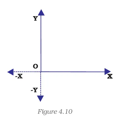
Two-dimensional (2-D) chart — A chart that presents data using two axes: the horizontal category axis and the vertical value axis.
| Axis | Direction | What it usually represents |
|---|---|---|
| -axis | Horizontal | Categories or independent values, such as months |
| -axis | Vertical | Data or derived values, such as demand |
Key points
- Axis: a line bordering the chart plot area that provides a measurement reference.
- Origin: the point where the -axis and -axis intersect.
- Positive and negative values: on the -axis, positive values are right of the origin and negative values left; on the -axis, positive values are above and negative values below.
- Example: profit may be plotted as a positive value and loss as a negative value.
Common 2-D chart types
- Types include line, bar, area, surface, column, multiple-line, radar, XY (scatter) and bubble charts.
- Column charts may be displayed horizontally or vertically, depending on the chart layout.
How should monthly product demand be plotted on a 2-D chart?
- Place the months, which are the independent categories, on the horizontal axis.
- Place the corresponding monthly demand values in rupees on the vertical axis.
Three-Dimensional Charts
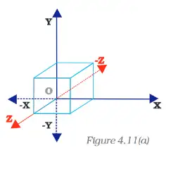
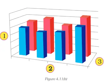
Three-dimensional (3-D) chart — A chart that adds a depth dimension, allowing data to be plotted along a third axis.
| Axis | Direction or role | Also called |
|---|---|---|
| -axis | Horizontal; categories | Category axis |
| -axis | Vertical; values | Derived-value axis |
| -axis | Depth; data series | Series axis |
Understanding the third dimension
- Volume example: volume uses height, length and breadth: height is represented on the -axis, length on the -axis, and breadth on the -axis.
- Use: the depth axis allows data series to be shown in addition to categories and values.
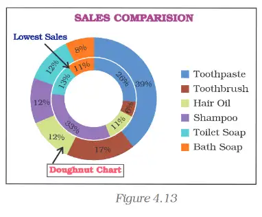
Radar, Pie and Doughnut Charts
Data series — A set of related data points plotted together, usually identified by its own colour or pattern and shown in the chart legend.
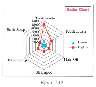
| Point | Radar | Pie | Doughnut |
|---|---|---|---|
| Main use | Compare aggregate values across data series | Show parts of a whole | Show parts of a whole; can display more than one series |
| Axes | No horizontal category axis | No axes | No axes |
| Series | Can compare multiple series | Has only one data series | Each ring represents a data series |
| Data layout | Data arranged in worksheet rows or columns | Data arranged in worksheet rows or columns | Data arranged in worksheet rows or columns |
Doughnut chart subtypes and use
- Doughnut: displays data in rings; each ring represents one data series.
- Exploded doughnut: separates or highlights individual values to emphasise their contribution to the total; it can show multiple series.
- Limitation: doughnut charts can be difficult to read; a stacked column or stacked bar chart may be clearer.
| Product | Lowest | Highest |
|---|---|---|
| Toothpaste | 2345 | 12344 |
| Toothbrush | 500 | 5415 |
| Hair Oil | 988 | 3678 |
| Shampoo | 2900 | 3770 |
| Toilet Soap | 1122 | 3861 |
| Bath Soap | 952 | 2344 |
| Total | 8807 | 31412 |
Advantages of Graphs and Charts
| Purpose | How charts help |
|---|---|
| Explore | Reveal possible relationships between variables quickly, without examining large amounts of raw data. |
| Present | Summarise and communicate information quickly and clearly. |
| Convince | Turn large amounts of information into visual evidence that can support persuasion. |
Which chart is suitable for comparing the lowest and highest sales values of several products?
A chart must show parts of a whole for more than one data series. What chart can be used, and what clearer alternative may be considered?
Quick recap
- Resize a selected chart by dragging a corner or border; chart text and other elements can be formatted independently.
- A 2-D chart uses the -axis for categories and the -axis for values; the axes meet at the origin.
- Positive and negative values appear on opposite sides of the origin on both axes.
- A 3-D chart adds the depth or series axis, the -axis; height maps to , length to , and breadth to .
- Radar charts compare data series; pie charts show one series as parts of a whole; doughnut charts can show multiple series as rings.
- Charts help users explore data, present information quickly and support persuasion.
Summary
Graphs and Chart Types
Graph — A graph is a pictorial representation of data, usually shown in two dimensions; three-dimensional graphs are also sometimes used.
| Point | Single-line graph | Multi-line graph |
|---|---|---|
| Lines shown | One data series | Two or more data series |
| Distinguishing series | Not needed | Use different line shapes or different line shapes and colours |
| Chart type | What it shows | Typical use |
|---|---|---|
| Pie chart | Relative share of different elements | Showing how a whole is divided among categories |
| Bar chart | Comparison of absolute data values | Comparing sales or production across products or time intervals |
Why Use Graphs and Charts?
- Visualisation: Graphs and charts make patterns and trends in data easier to see.
- Random data: They can make fluctuating data, such as stock prices, easier to understand than a textual description.
Chart Components in Excel
| Element | Purpose |
|---|---|
| Chart area | The overall area containing the chart and its elements |
| Plot area | The area where the selected chart type displays the data |
| Data points | The individual values represented in the chart |
| Horizontal axis | Usually shows base values, such as categories |
| Vertical axis | Usually shows derived values |
| Legend | Explains how lines, pie sections, bars or other series are distinguished |
| Chart and axis titles | Describe the chart and its axes |
| Data labels | Display values or other information beside data points |
Formatting and Display
- Formatting: Excel’s Design, Layout and Format options can modify chart elements, including the plot area, axes, data, titles, labels, legends and gridlines.
- Size: Resize a chart to suit the presentation.
- Chart type: Change the type, such as line to bar or bar to pie, when another view presents the data more effectively.
- Visibility: Axes, gridlines, legends, titles and data labels can be shown or hidden as needed.
Preparing a Chart
Create and Finish a Chart in Excel
- Enter the data in a worksheet with clear row and column titles.
- Select the data and create a basic chart using an option in the worksheet’s Chart group.
- Choose a predefined chart layout or style, and adjust the layout and formatting of chart elements.
- Add or remove the chart title, axis titles and data labels; a chart title can be linked to a worksheet cell.
- Show or hide the legend.
- Show or hide primary or secondary axes and gridlines.
- Move or resize the chart to fit the worksheet or presentation.
- Save the completed chart.
How can a chart be used to compare sales of several products in Excel?
- A worksheet lists sales for several products. Give a suitable chart and outline how to prepare it.
- Enter product names and sales values under clear column headings, then select the data.
- Choose a bar chart because the task is to compare absolute sales values across discrete product categories.
- Add a meaningful chart title and, if useful, axis titles or data labels; format the chart and show a legend if needed.
- Resize or move the chart as required and save it.
Which chart is generally suitable for showing the relative shares of different expense categories?
How can multiple data series be distinguished in a multi-line graph?
Quick recap
- Graphs pictorially represent data; they are usually two-dimensional.
- Pie charts show relative shares, while bar charts compare absolute values across categories or time intervals.
- Multi-line graphs distinguish series through line shapes and/or colours, with a legend explaining them.
- Excel charts include a chart area, plot area, data points, axes, legend, titles and data labels.
- Excel lets users format, resize and change chart types to improve presentation.
- Prepare charts by entering labelled data, selecting a chart, adjusting its elements and appearance, then saving it.
Formula sheet
Accountancy — ALL CHAPTERS
1
Accounting for Share Capital
2
Issue and Redemption of Debentures
3
Financial Statements of a Company
4
Analysis of Financial Statements
5
Accounting Ratios
6
Cash Flow Statement
1
Overview Of Computerised Accounting System
2
Spreadsheet
3
Use Of Spreadsheet In Business Applications
4
Graphs And Charts For Business Data
1
Accounting for Partnership: Basic Concepts
2
Reconstitution of a Partnership Firm –Admission of a Partner
3
Reconstitution of a Partnership Firm –Retirement/Death of a Partner
4
Dissolution of Partnership Firm