Class 12 Commerce . Accountancy . Computerised Accounting System . Spreadsheet
Chapter 2: Spreadsheet
Ch 2
Accountancy
Class 12 Commerce
Introduction
Spreadsheet: Structure and Purpose
Formula — A formula is an arithmetic expression and/or function that produces a derived value from other values.
Classify a value calculated from other spreadsheet values.
- A value entered directly is an independent value.
- A value obtained from other values using an arithmetic expression and/or function—a formula—is a derived value.
Spreadsheet Applications
- Purpose: Spreadsheet applications let users enter, organise, calculate and compare numerical or financial data.
- Worksheets: Data is arranged in rows and columns, and formulas or functions can calculate results from entered values.
Excel 2007 Interface
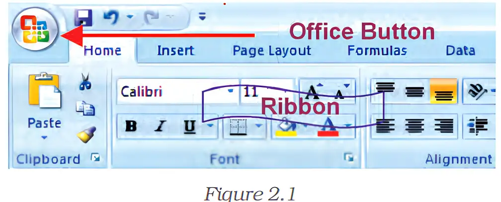
State the direction of rows and columns in a spreadsheet.
Name two actions available from the Office Button in Excel 2007.
Quick recap
- Spreadsheet: A grid of rows and columns for numerical or financial data.
- Rows and columns: Rows are horizontal; columns are vertical.
- Values: Independent values are entered directly; derived values are calculated using a formula.
- Formula: An arithmetic expression and/or function that produces a derived value.
- Spreadsheet application: A program for entering and processing data; MS Excel is an example.
- Excel 2007: The Ribbon provides tabs for accessing toolbars, and the Office Button provides workbook commands.
Basic Concepts Of Spreadsheet Part I
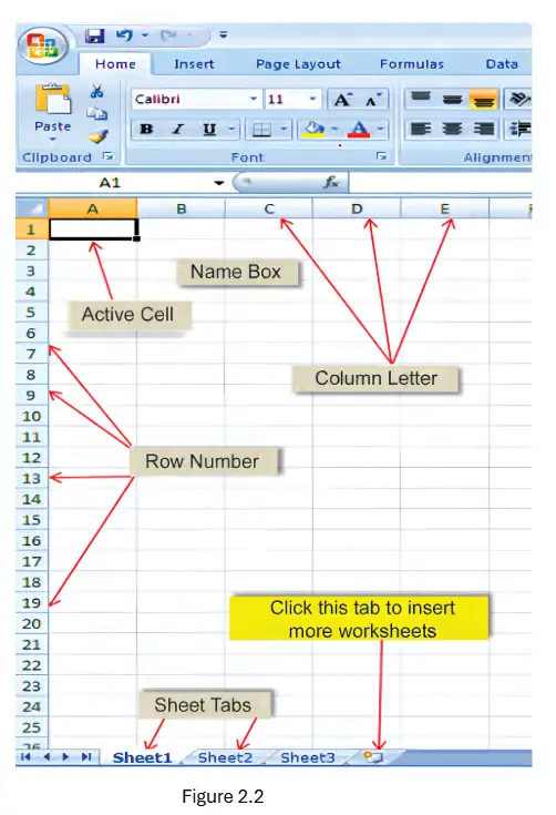
Workbooks and Worksheets
Basic and Derived Values
Quantity and price are basic values; the resulting item value is derived.
Find the value of 6 items priced at Rs. 25 each.
- An item has quantity 6 and price Rs. 25 per item. Substitute the basic values into the formula.
- Multiply quantity by price.
Rows, Columns and Worksheet Size
- Rows: Horizontal lines are numbered from top to bottom.
- Columns: Vertical lines are identified by letters from left to right.
- Excel 2007: Each worksheet has 65,536 rows and 256 columns, providing about 16.5 million cells.
Cell Address and Cell Reference
| Reference type | Example | What happens when copied? |
|---|---|---|
| Relative | `C4` | The row and column references adjust to the formula's new location; this is the default. |
| Absolute | `4` | Both column and row stay fixed. |
| Mixed | `4` | One part stays fixed: `4` fixes the row. |
Moving Around a Worksheet
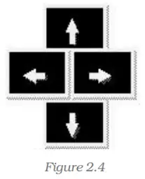
| Movement | Key |
|---|---|
| One cell down | Down Arrow or Enter |
| One cell up | Up Arrow |
| One cell left | Left Arrow |
| One cell right | Right Arrow or Tab |
| Movement | Key |
|---|---|
| Go to the top of the worksheet (`A1`) | CTRL + HOME |
| Go to the last row and column containing data | CTRL + END |
| Move through filled-cell boundaries in a row | Successive CTRL + Right Arrow, or END + Right Arrow |
| Move through filled-cell boundaries in a column | Successive CTRL + Down Arrow, or END + Down Arrow |
| Go to the beginning of the current row | HOME |
Data Entered in a Cell
Classify the inputs `125`, `North Zone` and `28/10/2026` as numeric, alphanumeric or date data.
A formula in `D5` refers to `C4`. State how the reference behaves if copied one cell down and one cell right. How would you write it to keep the reference fixed?
Quick recap
- A workbook contains worksheets; only one worksheet is active at a time.
- Rows are numbered and columns are lettered; their intersection is a cell.
- Cell addresses combine a column letter and row number; a range uses a colon between its endpoints.
- Relative references adjust when copied, absolute references stay fixed, and mixed references fix one part.
- Arrow keys move one cell; CTRL + HOME and CTRL + END support faster navigation.
- Cell entries may be numeric, alphanumeric or dates; basic values can be used to calculate derived values.
Basic Concepts Of Spreadsheet Part II
Cell Values and Planning
- Cell contents: A cell may contain a number, text, date, formula or function.
- Data types: Excel recognises entries such as 306 as numeric, Asset as alphanumeric and 12/07/08 as a date.
- Planning: Decide which cells will hold input values and which cells will contain relationships or calculations.
- Basic and derived values: Enter basic values directly; formulas use them to calculate derived values, which update when inputs change.
- What-if analysis: Change one or more input values to examine their effect on calculated results.
Basic Concepts Of Spreadsheet Part III
Spreadsheet Functions
Enter the function name and its argument(s) after the equal sign.
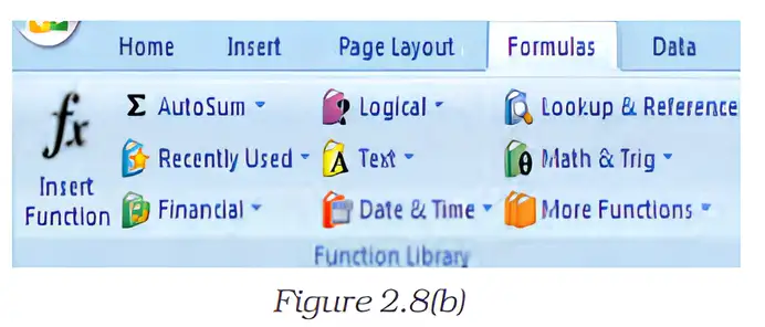
Function Tools and Categories
- AutoSum (∑): Inserts a SUM formula quickly; its menu also offers AVERAGE, MIN, MAX and COUNT.
- Excel 2007: Has 12 function categories. Categories especially useful in computerised accountancy include Financial, Date and Time, Lookup and References, Database, Text and Logical.
Using AutoSum
- Select the cell where the total should appear.
- Click AutoSum and check or enter the range to add.
- Confirm the formula; the total appears in the selected cell.
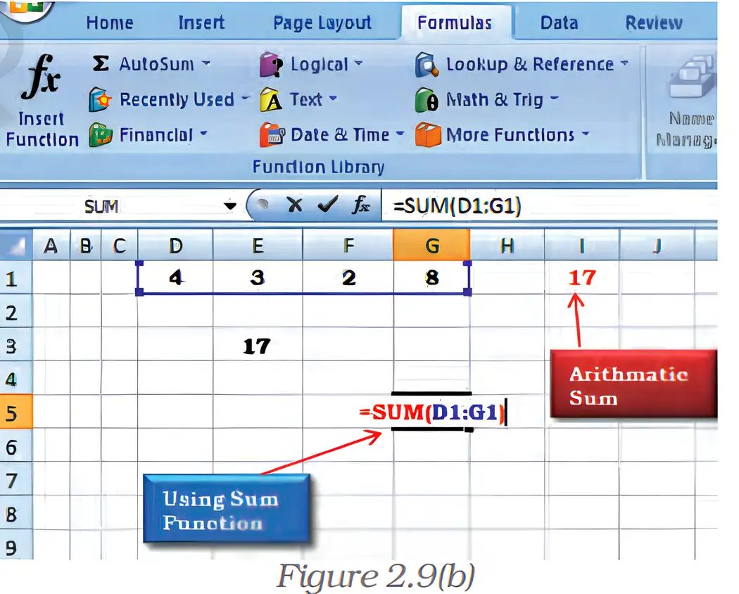
Find the total of the values in D1:G1, whose sum is 17.
- To total cells D1:G1 in H1, enter the SUM formula.
- The values in the range add to 17, which is displayed in H1.
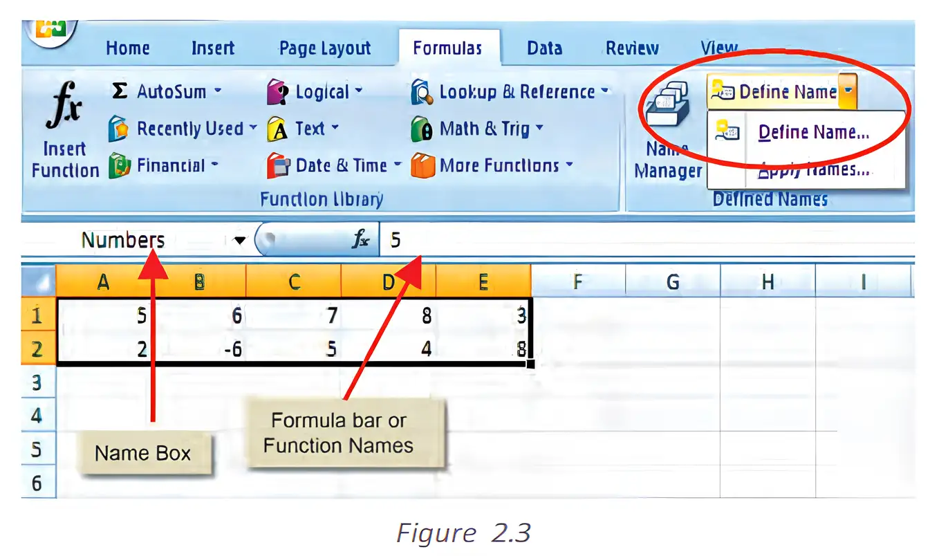
Naming Cells and Ranges
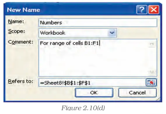
Use the defined name in place of the range address.
Define and use a named range
- Select the cell or range to name.
- On the Formulas tab, choose Define Name.
- Enter the name and check the range shown in Refers to; click OK.
- Use the name in a formula. Apply Names can insert an existing name in place of cell references.
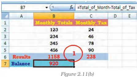
Use the named ranges Monthly_Totals and Monthly_Tax to calculate their totals.
- Monthly_Totals refers to B2:B5; use it to calculate the total in B6.
- Monthly_Tax refers to C2:C5; use it to calculate the total in C6.
- The formulas return the stated totals.
Conditional Summation with SUMIF
This form totals values in the named range that meet the criterion.
What is the result of summing the values in Numbers that are less than 6?
- Numbers is the named range to test; the criterion is less than 6.
- Add only the values in Numbers that meet the criterion.
What does =COUNT(A1:A8) count?
Cells B2:B5 are named Monthly_Totals. Write a formula to calculate their average.
Do not treat text cells as numeric inputs for SUM, AVERAGE or COUNT; these functions use numbers and ignore blank or text cells in the described ranges. Write comparison criteria in quotation marks, for example =SUMIF(Numbers,"<6").
Quick recap
- Functions are built-in formulas that begin with an equal sign and process arguments to return results.
- SUM adds numbers; AVERAGE finds their mean; COUNT counts numeric cells; MIN and MAX return the smallest and largest values.
- AutoSum inserts a SUM formula quickly and provides other common function choices.
- Excel 2007 provides 12 function categories, including several useful in computerised accountancy.
- Named ranges replace cell references with descriptive names in formulas.
- SUMIF adds only values that satisfy a condition; the example totals values less than 6 to get 9.
Basic Concepts Of Spreadsheet Part IV
Named Ranges, Balances, and Freezing Values
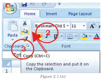
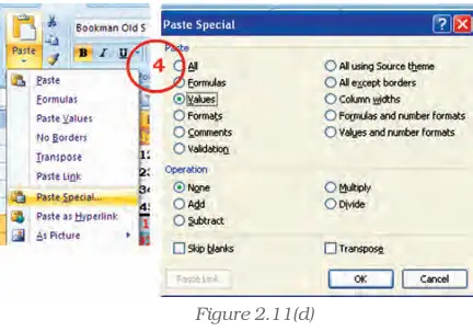
Freeze formulas using Paste Special
- Select the formula cells, such as and .
- Copy the selected cells.
- Choose Paste Special and select Values.
- Confirm. The formulas are replaced by their current calculated values.
IF Function
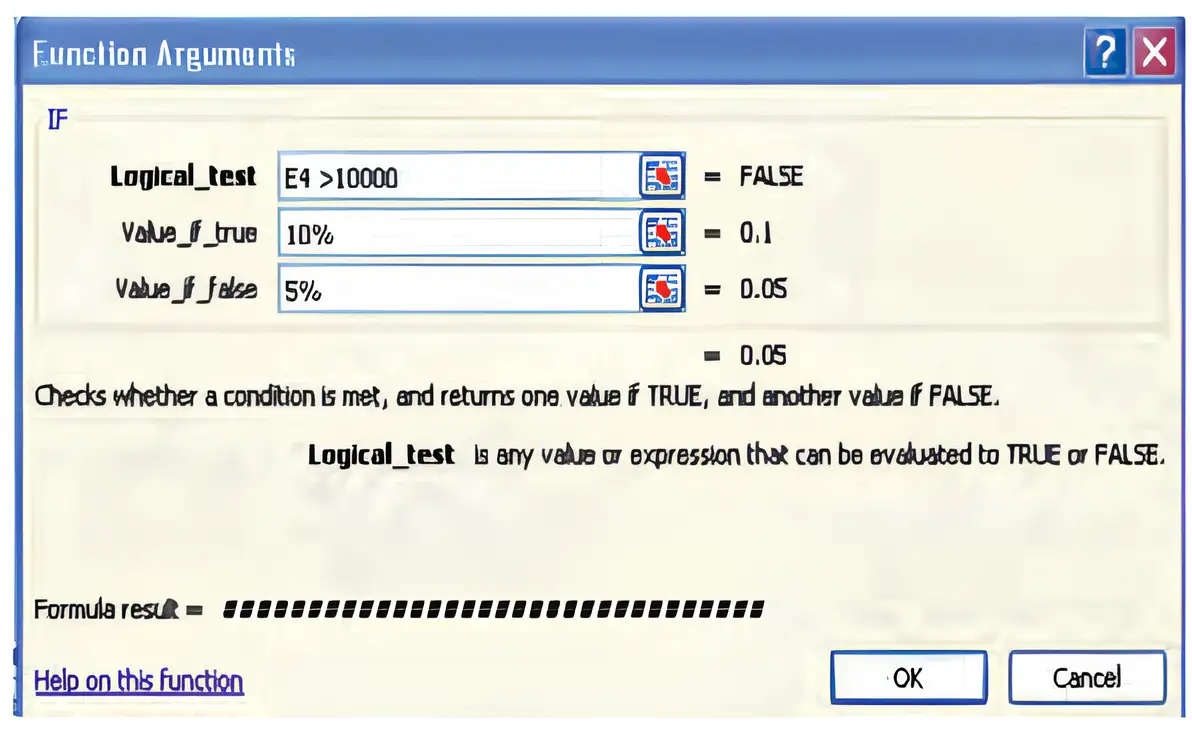
Use this structure to return one result for a TRUE test and another for a FALSE test.
IF examples
- Text result: To show Yes when and No otherwise, use ; text results must be enclosed in quotation marks.
- Different calculations: returns the first average if ; otherwise it returns the second.
- Combined functions: sums when the average of exceeds ; otherwise it returns .
Using IF for a saving percentage
- Condition: If the total in exceeds , return a saving rate of ; otherwise, return .
- Formula: In , enter and copy it down for the other rows.
- Amount: Multiply the total by the selected rate; for example, .
If , what saving rate and amount does the formula return?
- For a total of in , test whether it exceeds .
- The IF formula returns a rate of .
Nested IF Functions
For marks in , the formula checks thresholds in order; text results are enclosed in quotation marks.
| Marks | Result |
|---|---|
| Below | Fail |
| to below | C Grade |
| to below | B Grade |
| or more | A Grade |
What grade does the nested IF formula return when ?
- For , check the first condition.
- Check the next condition; it is false, so the formula returns the B Grade result.
Write an IF formula that returns Yes if and No otherwise.
If , what result does the nested grade formula return?
Quick recap
- Named ranges make formulas easier to read; subtract named tax from the named monthly total to calculate a balance.
- Paste Special → Values replaces formulas with their current results, stopping later recalculation.
- IF returns one result for TRUE and another for FALSE; text results need quotation marks.
- Logical operators compare values and produce TRUE or FALSE.
- IF examples can return text, different calculations, or results from functions such as AVERAGE and SUM.
- Nested IFs test conditions in sequence; the final FALSE result handles cases not matched earlier.
Basic Concepts Of Spreadsheet Part V
Other Useful Functions
Function libraries
- Purpose: Spreadsheet functions use input data as arguments and return calculated information, such as ages, payment delays, interest, depreciation, or future values.
- Categories: Date and Time; Mathematical; Text Manipulation; Logical (other than IF); Lookup and Reference; Financial.
- Help: Use Excel Help for function details. Typing a function name after `=` and selecting it from the suggestion strip is a quick way to access help.
Date and Time Functions
Excel date serial number — Excel stores dates as serial numbers for calculations; times are stored as fractions of a day. January 1, 1900 is serial number 1, and January 1, 2009 is serial number 39814.
Date and time function outputs
- TODAY(): Returns the serial number of the current date.
- NOW(): Returns the current date and time.
- DAY(serial_number): Returns the day of the month as an integer from 1 to 31.
- MONTH(serial_number): Returns the month as an integer from 1 to 12; April returns 4.
- YEAR(serial_number): Returns the year as an integer from 1900 to 9999.
- DATEVALUE(date_text): Converts a text-form date into its Excel date serial number; for example, `=DATEVALUE("16-04-2009")` returns 39919.
Use `=DAY(A1)`, `=MONTH(A1)` or `=YEAR(A1)` to extract a date part. Approximate age in years by dividing the date difference by 365.25, allowing for leap years.
Estimate age from two dates
- Subtract the date-of-birth serial number from the later date's serial number.
- Divide the elapsed days by 365.25 to estimate age in years.
Find the approximate age on 16-Apr-2009 of a person born on 16-Apr-1980.
- Estimate the age on 16-Apr-2009 of a person born on 16-Apr-1980; their serial numbers are 39919 and 29327.
- Convert elapsed days to years.
- Interpret the approximate result.
Mathematical Functions
SUMIF — Adds values from cells whose corresponding entries meet a specified condition.
The range is tested against the criterion; the optional sum_range contains the values to add. If sum_range is omitted, Excel sums the tested range itself.
| Asset value | Depreciation |
|---|---|
| Rs. 100,000 | Rs. 7,000 |
| Rs. 200,000 | Rs. 14,000 |
| Rs. 300,000 | Rs. 21,000 |
| Rs. 400,000 | Rs. 28,000 |
| Total | Rs. 70,000 |
Apply SUMIF
- Set range to the cells being tested and criteria to the condition.
- Set sum_range to the corresponding values to add.
Using the table, find total depreciation for assets valued above Rs. 150,000.
- Select depreciation for assets valued above Rs. 150,000.
- The qualifying assets are Rs. 200,000, Rs. 300,000 and Rs. 400,000; add their depreciation.
For the asset example, test `D2:D5` and sum the matching cells in `E2:E5`; do not use the two-column range `D2:E5` as the criteria range.
ROUND — Rounds a number to a specified number of digits.
A positive num_digits rounds to decimal places; zero rounds to the nearest integer; a negative value rounds to the left of the decimal point.
ROUNDUP rounds away from zero; ROUNDDOWN rounds toward zero. All three functions use num_digits to set the rounding place.
| Formula | Result |
|---|---|
| `=ROUND(2.15,1)` | 2.2 |
| `=ROUND(2.149,1)` | 2.1 |
| `=ROUND(-1.475,2)` | -1.48 |
| `=ROUND(21.5,-1)` | 20 |
| `=ROUNDUP(3.2,0)` | 4 |
| `=ROUNDUP(76.9,0)` | 77 |
| `=ROUNDUP(3.14159,3)` | 3.142 |
| `=ROUNDUP(-3.14159,1)` | -3.2 |
| `=ROUNDUP(31415.92654,-2)` | 31,500 |
| `=ROUNDDOWN(3.2,0)` | 3 |
| `=ROUNDDOWN(76.9,0)` | 76 |
| `=ROUNDDOWN(3.14159,3)` | 3.141 |
| `=ROUNDDOWN(-3.14159,1)` | -3.1 |
| `=ROUNDDOWN(31415.92654,-2)` | 31,400 |
Round a number
- Choose the required rounding place using num_digits.
- Use ROUND for ordinary rounding, ROUNDUP to move away from zero, or ROUNDDOWN to move toward zero.
Compare ROUND, ROUNDUP and ROUNDDOWN for 31415.92654 with num_digits -2.
- Round 31415.92654 to the nearest hundred with ROUND.
- ROUNDUP moves away from zero to the next hundred.
- ROUNDDOWN moves toward zero to the previous hundred.
Cell A1 contains the date 16-Apr-2009. What do `=DAY(A1)`, `=MONTH(A1)` and `=YEAR(A1)` return?
What is `=ROUNDUP(-3.14159,1)`?
Using the asset table, what does `=SUMIF(D2:D5,">250000",E2:E5)` return?
Quick recap
- Excel functions take arguments and return calculated results; useful groups include Date and Time, Mathematical, Text Manipulation, Logical, Lookup and Reference, and Financial.
- Dates are serial numbers and times are fractions of a day; January 1, 1900 is serial 1 and January 1, 2009 is serial 39814.
- TODAY returns the current date, while NOW includes the time; DAY, MONTH and YEAR extract date components, and DATEVALUE converts a text date to a serial number.
- Approximate age in years is the difference between date serials divided by 365.25.
- SUMIF tests a range against a criterion and adds corresponding cells in the optional sum_range.
- ROUND uses num_digits to choose the rounding place; ROUNDUP moves away from zero and ROUNDDOWN moves toward zero.
Basic Concepts Of Spreadsheet Part VI
Counting Functions
Count_Data contains 18 total cells, 13 occupied cells, and 7 numeric entries. Find the number of blanks and the COUNT result.
- Find blanks by subtracting occupied cells from the total.
- Use the sample's reported numeric-entry count for COUNT.
Array Dimensions and Array Formulas
Find the number of cells in A1:C4.
- Find the number of rows and columns in A1:C4.
- Multiply the dimensions to find the cell count.
COUNTIF
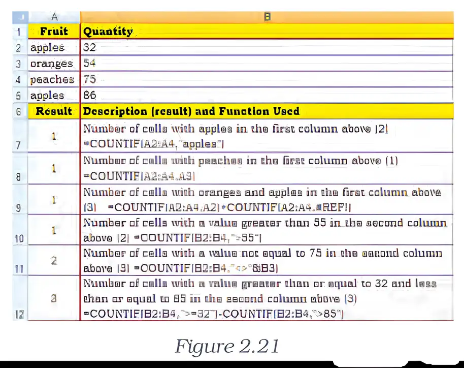
A2:A6 contains 10, 32, 40, 32, and 25. Count the values greater than 30.
- Apply COUNTIF to A2:A6 with the condition greater than 30.
- Three entries satisfy the condition: 32, 40, and 32.
- Therefore, the function returns 3.
Text Manipulation: TEXT
L1 contains 23.5. Use TEXT to display the value as Rs. 23.50.
- Format the value in L1 with two decimal places and the rupee label.
- The function returns formatted text.
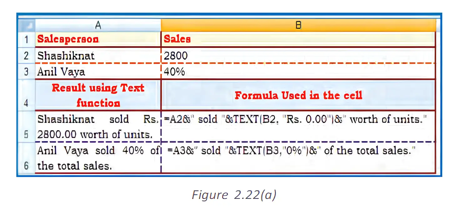
Do not confuse COUNT and COUNTA: COUNT counts numeric entries; COUNTA counts every nonblank cell, including text, logical values, and errors.
Do not treat TEXT as cell formatting: TEXT returns text, while number-formatting commands change the appearance of numeric cells; those commands work only when the entire cell is numeric.
A1:A5 contains apples, pears, apples, a blank cell, and oranges. How many cells contain apples?
A range has 5 rows and 2 columns. How many cells does it contain?
Cell B2 contains 8.4. Use TEXT to display it with two decimal places.
Quick recap
- COUNT counts numeric entries, including dates; directly supplied values may include numeric text or logical values, while text and logical values in references or arrays are ignored.
- COUNTA counts nonblank cells; COUNTBLANK counts blanks; COUNTIF counts cells meeting a criterion.
- ROWS and COLUMNS return array dimensions; multiply them to find the total number of cells.
- Array formulas perform multiple calculations and return one or more results; traditional entry uses Ctrl+Shift+Enter and braces.
- TEXT converts a number to formatted text, such as 23.5 becoming Rs. 23.50.
- Home-tab number formatting changes the appearance of a numeric cell; it works only if the entire cell is numeric.
Basic Concepts Of Spreadsheet Part VII
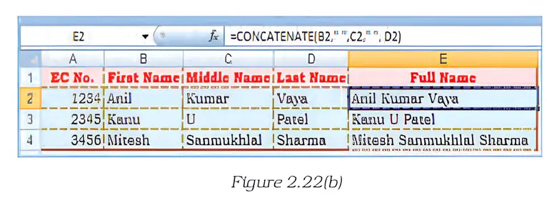
CONCATENATE Function
CONCATENATE — Joins two or more text items into one text string.
Key points
- Arguments: Takes 2 to 255 items, such as text strings, numbers, or single-cell references.
- Output: Combines the items in the order supplied.
- Spaces: Add a space as a separate text item when needed; CONCATENATE does not add spaces automatically.
Use text strings, numbers, or single-cell references as the items to join.
Combine name fields
- Select the cells containing the name parts.
- Place a space string between the cell references.
- Join the parts with CONCATENATE.
How can the first, middle, and last names in A2, B2, and C2 be combined?
- Suppose A2, B2, and C2 contain the first, middle, and last names.
- Join the three cells with spaces between them.
- The function returns the full name.
Logical Functions
Logical value — A result of TRUE or FALSE produced by comparing values or arithmetic expressions.
AND Function
AND — Returns TRUE only when every argument evaluates to TRUE; otherwise, it returns FALSE.
Key points
- Arguments: Takes up to 255 logical tests, including comparisons or expressions.
- TRUE result: Every argument must be TRUE.
- FALSE result: One or more arguments are FALSE.
- With IF: Using AND as IF's logical test lets IF check several conditions together.
Each logical argument is a condition to test.
Test whether a value is in a range
- Write one comparison for the lower limit and one for the upper limit.
- Combine both tests with AND.
- To return a value or message, use AND inside IF.
If A2 contains 50, what does `=IF(AND(A2>1,A2<100),A2,"The value is out of range.")` return?
- A2 contains 50; test whether it is greater than 1 and less than 100.
- Both comparisons are TRUE, so AND returns TRUE.
- With IF, the value in A2 is returned because the combined test is TRUE.
| Formula | Result | Reason |
|---|---|---|
| `=AND(TRUE,TRUE)` | TRUE | All arguments are TRUE. |
| `=AND(TRUE,FALSE)` | FALSE | At least one argument is FALSE. |
| `=AND(2+2=4,2+3=5)` | TRUE | Both expressions are TRUE. |
OR Function
OR — Returns TRUE when at least one argument is TRUE; it returns FALSE only when every argument is FALSE.
Key points
- Arguments: Takes up to 255 logical tests.
- TRUE result: One or more arguments are TRUE.
- FALSE result: All arguments are FALSE.
Each logical argument is a condition to test.
Combine alternative conditions
- Enter each acceptable condition as a logical argument.
- Use OR to test whether at least one condition is satisfied.
What does `=OR((1+1)=1,(2+2)=5)` return?
- Evaluate the two comparisons.
- Since both arguments are FALSE, OR returns FALSE.
| Formula | Result | Reason |
|---|---|---|
| `=OR(TRUE,FALSE)` | TRUE | At least one argument is TRUE. |
| `=OR((1+1)=1,(2+2)=5)` | FALSE | All arguments are FALSE. |
| `=OR(TRUE,FALSE,TRUE)` | TRUE | At least one argument is TRUE. |
LOOKUP Function
LOOKUP — Searches a range or array for a value and returns a corresponding value from another position.
Two forms
- Vector form: Searches a single-row or single-column lookup range and returns the value at the same position in a second single-row or single-column range.
- Array form: Searches the first row or column of an array and returns a value from the corresponding position in its last row or column.
- Use: LOOKUP can be an alternative to elaborate IF tests or tests that exceed IF nesting limits.
LOOKUP — Vector Form
Arguments and rules
- lookup_value: The number, text, logical value, name, or reference being searched for.
- lookup_vector: A one-row or one-column range; its values must be in ascending order.
- result_vector: A one-row or one-column range with the same size as lookup_vector.
- Approximate match: If no exact match is found, LOOKUP selects the largest lookup value less than or equal to the search value.
- Below the range: If lookup_value is smaller than the smallest lookup value, LOOKUP returns #N/A.
The lookup and result vectors must have the same number of items.
| Frequency (A) | Colour (B) |
|---|---|
| 4.14 | red |
| 4.19 | orange |
| 5.17 | yellow |
| 5.77 | green |
| 6.39 | blue |
Use vector LOOKUP
- Check that the lookup vector is in ascending order.
- Specify the search value, lookup vector, and same-sized result vector.
- Read the corresponding result for the exact or next-smallest match.
What does `=LOOKUP(7.66,A2:A6,B2:B6)` return for the given frequency and colour data?
- Search for 7.66 in the ascending frequency vector.
- The largest frequency not greater than 7.66 is 6.39.
- The colour in the matching position is blue.
| Formula | Result | Reason |
|---|---|---|
| `=LOOKUP(4.19,A2:A6,B2:B6)` | orange | Exact match at 4.19. |
| `=LOOKUP(5.00,A2:A6,B2:B6)` | orange | 4.19 is the largest lookup value not greater than 5.00. |
| `=LOOKUP(7.66,A2:A6,B2:B6)` | blue | 6.39 is the largest lookup value not greater than 7.66. |
| `=LOOKUP(0,A2:A6,B2:B6)` | #N/A | 0 is less than the smallest lookup value, 4.14. |
Do not use an unsorted lookup vector or vectors of different sizes: the result may be incorrect, and the result vector must match the lookup vector in size.
A3 contains 104. What does `=IF(AND(A3>1,A3<100),A3,"The value is out of range.")` return?
What does `=OR(TRUE,FALSE,TRUE)` return?
Using the frequency and colour table, what does `=LOOKUP(5.00,A2:A6,B2:B6)` return?
Quick recap
- CONCATENATE joins 2 to 255 items; add a separate space string when names need spaces.
- AND returns TRUE only when all its logical arguments are TRUE.
- OR returns TRUE when at least one logical argument is TRUE.
- IF with AND tests several conditions and returns a value or a message based on the combined result.
- LOOKUP vector form searches one row or column and returns the corresponding item from a same-sized result vector.
- LOOKUP matching requires ascending lookup values and uses the largest value less than or equal to the search value; a value below the range returns #N/A.
Basic Concepts Of Spreadsheet Part VIII
LOOKUP: Array Form
LOOKUP (array form) — Searches an array for a value and returns a corresponding value from the array’s opposite edge.
Key rules
- Lookup value: May be a number, text, logical value, or a reference/name that points to a value.
- Search direction: If the array is wider than it is tall, LOOKUP searches its first row; otherwise, it searches its first column.
- Return value: For a wide array it returns from the last row; for a square or tall array, it returns from the last column.
- Approximate match: If the exact value is absent, LOOKUP uses the largest value less than or equal to the lookup value.
- Error: Returns #N/A if the lookup value is smaller than the smallest value in the search row or column.
Use the array form to search an entire rectangular range.
Using LOOKUP with an array
- Identify the lookup value and the array range.
- Determine whether the array is wider than it is tall.
- Search the first row if wide; otherwise search the first column.
- Return the corresponding value from the last row or last column.
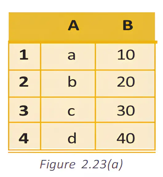
What does =LOOKUP("c",A1:B4) return when column A contains a, b, c, d and column B contains 10, 20, 30, 40?
- In A1:B4, the range is taller than it is wide, so LOOKUP searches column A and returns the corresponding value from column B.
- Searching for c matches the third entry in column A.
- The corresponding value in column B is 30.
Do not assume LOOKUP always searches the first column: the array’s shape decides whether it searches the first row or first column.
VLOOKUP
VLOOKUP — Searches vertically in the first column of a table and returns a value from another column in the matching row.
Here, v is the lookup value, T is the table range, c is the return-column index, and r specifies the match type. The column index is counted from the first column of the selected table.
Arguments and results
- lookup_value: Value or reference searched for in the table’s first column; if it is below the smallest value, the result is #N/A.
- table_array: Range with at least two columns; its first column contains the values to search. Uppercase and lowercase text are treated as equivalent.
- col_index_num: Column to return from the selected table; 1 returns its first column, 2 its second, and so on.
- Invalid column index: An index below 1 returns #VALUE!; an index greater than the table’s column count returns #REF!.
- range_lookup = TRUE or omitted: Allows approximate matching; the first column must be sorted in ascending order. An exact match is used when available; otherwise the next smaller value is returned.
- range_lookup = FALSE: Requires an exact match; sorting is not required. If duplicates exist, the first match is used; no match returns #N/A.
| Employee Code | First Name | Last Name | Basic Pay (Rs.) |
|---|---|---|---|
| 1873 | Prakash | Sharma | 5,176.00 |
| 3456 | Shaashikant | Thakur | 3,453.00 |
| 4537 | Ajit | Mathur | 3,355.00 |
| 5678 | Vinod | Upadhyay | 428.00 |
| 16782 | Kanu | Patel | 3,457.00 |
| 34567 | Anil | Vaya | 5,467.00 |
Using VLOOKUP
- Choose the lookup value and a table range whose first column contains it.
- Set the column index to the position of the value to return.
- Use FALSE for an exact match or TRUE for an approximate match.
- Check the returned value in the same row as the match.
Find the basic pay for employee code 3456 using the employee table.
- Search for employee code 3456 in the first column and request the fourth column with an exact match.
- The matching row contains a basic pay of Rs. 3,453.00 in column 4.
| Item ID | Item | Cost (Rs.) | Markup |
|---|---|---|---|
| AS-469 | Aspirator | 2.56 | 45% |
| BI-567 | Bib | 3.56 | 40% |
| DI-328 | Diapers | 21.45 | 35% |
| ST-340 | Stroller | 145.67 | 30% |
| WI-989 | Wipes | 5.12 | 40% |
VLOOKUP in calculations
- Retail price: Multiply cost by one plus the markup rate; for DI-328, the price is (rounded).
- Discounted sale price: Multiply cost by one plus markup, then by one minus the discount; WI-989 with a 20% discount gives (rounded).
- Conditional message: IF can test whether the looked-up cost is at least Rs. 20 and display the markup; otherwise, it can report the cost or that it is under Rs. 20.
The examples use exact-match lookups; multiply the looked-up cost by the markup and discount factors.
Using LOOKUP array form, what is returned for lookup value b in A1:B4, where the first column is a, b, c, d and the second is 10, 20, 30, 40?
Find the retail price of diapers (DI-328) using the product table.
A product costs Rs. 3.56 and has a 40% markup. What message should an IF test with a Rs. 20 cost threshold display?
Quick recap
- LOOKUP array form: Searches the first row of a wide array or first column of a square/tall array.
- LOOKUP result: Returns the corresponding value from the opposite edge; if no exact value exists, it uses the largest value not exceeding the lookup value.
- VLOOKUP: Searches the table’s first column and returns a value from the matching row.
- Column index: Counts from the first column of the selected table; invalid indices return #VALUE! or #REF!.
- Match setting: FALSE requires an exact match; TRUE or omission permits approximate matching and requires ascending order.
Basic Concepts Of Spreadsheet Part IX
HLOOKUP
HLOOKUP — HLOOKUP (Horizontal Lookup) searches the first row of a table array and returns a value from another row in the same column.
HLOOKUP arguments and rules
- Lookup value — The value to search for in the table array’s first row.
- Table array — A range with at least two rows; the first row may contain text, numbers, or logical values. Text matching is not case-sensitive.
- Row index number — The row within the selected table array from which to return a value; for example, means its second row.
- Range lookup — FALSE requires an exact match. TRUE allows the nearest match when no exact match is found and generally requires the first row to be sorted in ascending order.
- Copying formulas — Make the table-array reference absolute so it does not shift when the formula is copied.
Use FALSE when the lookup must match exactly.
Using HLOOKUP
- Select the value to look up from the table’s first row.
- Select the complete table range and lock its cell references before copying the formula.
- Enter the row number containing the result and choose FALSE for an exact match.
- Retrieve the matching quarter’s budget, then subtract the amount spent to find the pending budget.
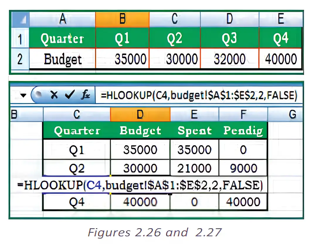
How can the budget for the quarter in C4 be retrieved and its pending amount calculated?
- In D4, find the quarter named in C4 and return its budget from the second row of the Budget worksheet’s table.
- In F4, subtract the amount spent in E4 from the retrieved budget.
Do not confuse the row index with a column number: HLOOKUP returns from the specified row of the table array. Lock the table range before copying the formula.
Financial Functions
- Purpose: Financial functions calculate values used in investments, loans and other financial applications.
- Inputs: Their arguments can include an interest rate, number of periods, payments and present or future values.
- Applications: Excel provides functions for interest, loan payments, investment values and net present value.
ACCRINT
ACCRINT — ACCRINT calculates accrued interest for a security that pays interest periodically.
ACCRINT arguments and dates
- Issue — The security’s issue date; first_interest — The date of its first interest payment.
- Settlement — The date after issue when the security is traded to the buyer.
- Rate — The annual coupon rate; par — The security’s par value, defaulting to Rs. 1,000.
- Frequency — Coupon payments per year: annual , semi-annual , and quarterly .
- Basis — The day-count basis used; calc_method — The calculation-method argument.
- Date inputs — Use actual date values, preferably with the DATE function; text dates can cause problems.
- Date serials — Spreadsheet dates are stored as sequential numbers: January 1, 1900 is serial , and January 1, 2008 is serial .
Enter dates as date values, not text.
Here, is the number of coupon periods; is the fraction of period accrued.
Preparing an ACCRINT calculation
- Enter the issue, first-interest, and settlement dates as date values.
- Supply the annual rate, par value, payment frequency, basis, and calculation method.
- Use the returned value as the accrued interest for the security.
How should May 23, 2008 be entered as a date for an ACCRINT calculation?
- To enter May 23, 2008 as a date value, use the DATE function.
- Use this date in the appropriate date argument of ACCRINT; the example date alone does not identify which date argument it represents.
CUMIPMT
CUMIPMT — CUMIPMT returns the cumulative interest paid over a selected range of payment periods.
CUMIPMT arguments
- Rate — Interest rate per payment period; nper — Total number of payment periods.
- pv — Present value of the loan.
- Start period and end period — First and last periods included; payment periods are numbered from .
- Type — Payment timing: means end of period and means beginning of period.
- Returned sign — Interest paid is commonly returned as a negative cash flow.
Use the rate and number of periods in the same payment-period units.
Using CUMIPMT
- Convert the annual interest rate and loan term to the payment-period units.
- Enter the present value and the first and last periods to include.
- Set type to 0 for end-of-period payments or 1 for beginning-of-period payments.
What is the cumulative interest for periods 13–24 on a 30-year loan of Rs. 125,000 at an annual interest rate of 9%, with end-of-month payments?
- Convert the annual rate to a monthly rate and the 30-year term to monthly periods.
- Select periods 13 through 24 and use type 0 for payments at the end of each month.
- For the loan present value of Rs. 125,000, the function returns the second year’s total interest.
A table has quarter names in its first row and budgets in its second row. Which HLOOKUP row index returns a budget?
What frequency should be used for a security that pays interest quarterly?
Using the loan data in the example, find the interest for the first month when payments are made at period end.
Quick recap
- HLOOKUP searches the first row and returns a value from the specified row in the matching column.
- Use FALSE for an exact HLOOKUP match; use an absolute table-array reference when copying formulas.
- ACCRINT calculates accrued interest using security dates, coupon rate, par value, frequency, basis, and calculation method.
- Enter ACCRINT dates as date values, such as with the DATE function, rather than as text.
- CUMIPMT calculates cumulative interest for a selected range of payment periods.
- For CUMIPMT, match the rate and total periods to the payment frequency; type 0 means end-of-period payments and type 1 means beginning-of-period payments.
Basic Concepts Of Spreadsheet Part X
Present Value (PV)
Use the and arguments when needed. If is omitted, must be supplied; if is omitted, must be supplied.
For a non-zero periodic rate, the present value, payments and future value balance to zero when cash-flow signs are entered consistently.
Use this special case when the periodic interest rate is zero.
What is the present value of the payment series?
- Find the present value of monthly payments of Rs. 500 for 20 years at an annual interest rate of 8%, paid at each month's end.
- Convert the annual rate and years into monthly terms.
- Use the payment as a positive cash flow; the calculated present value has the opposite sign.
Do not pair an annual rate with a monthly period count: convert both to the same time unit. Also, a negative PV result may simply reflect the cash-flow sign convention.
Future Value (FV)
If is omitted, include ; if is omitted, include .
FV balances the grown present value and accumulated payments, with cash-flow signs entered consistently.
At a zero rate, the future value is the opposite of the present value plus all payments.
How does the payment timing affect the result?
- Find the future value using a monthly rate of 6% per year divided by 12, 10 periods, payments of Rs. 200 and a present value of Rs. 500; payments are at the beginning of each period.
- Enter the payment and present value as negative cash flows, and set the payment timing to the beginning of the period.
- Changing only the payment timing to the end of each period gives a lower future value.
Do not confuse (the initial amount) with (the final balance). Use consistent cash-flow signs and the correct payment timing.
What is the present value of 12 end-of-period payments of Rs. 100 when the periodic rate is zero?
Find the future value after 12 end-of-period payments of Rs. 100 and an initial investment of Rs. 500, when the periodic rate is zero.
Quick recap
- PV calculates the current worth of future annuity payments; FV calculates an investment's value at the end.
- Match the rate period to the payment-period count.
- Payments are fixed across periods and usually include principal and interest, not fees or taxes.
- For PV, omitted requires ; omitted requires .
- For FV, omitted requires ; omitted requires .
- means end-of-period payments; means beginning-of-period payments.
- Use positive and negative cash flows consistently; the calculated balancing value may have the opposite sign.
Basic Concepts Of Spreadsheet Part XI
PMT Function
PMT function — Calculates the equal periodic payment for an annuity or loan when the interest rate is constant.
Arguments and use
- rate is the interest rate per payment period; convert an annual rate to match the payment frequency.
- nper is the total number of payment periods; pv is the present value or loan amount.
- fv is the balance desired after the last payment; if omitted, it is assumed to be zero.
- type is or omitted for end-of-period payments and for beginning-of-period payments.
- Use: PMT is commonly used to calculate fixed mortgage or loan payments.
Match the rate and period count to the payment frequency.
Find the monthly payment for both payment timings.
- For a Rs. 10,000 loan at 8% annually with monthly payments over 10 months, convert the rate to a monthly rate.
- Use the default type for payments at each month-end.
- Set type to 1 for payments at each month-beginning.
Do not use the annual rate directly with monthly payments: divide it by and use the total number of months for nper.
RATE Function
RATE function — Finds the interest rate per period of an annuity from its payment and present or future value.
Arguments and calculation
- nper is the total number of payment periods; pmt is the fixed payment each period.
- pv is the present value; fv is the balance after the last payment and defaults to zero.
- If pmt is omitted, include fv as an argument.
- type is or omitted for end-of-period payments and for beginning-of-period payments; guess is the starting estimate and defaults to .
- Iteration: RATE may have zero or more solutions. If results do not converge within after iterations, it returns #NUM!.
RATE returns the rate per payment period. For monthly payments, multiply the monthly rate by to obtain a nominal annual rate.
Find the monthly rate and nominal annual rate for the loan.
- A four-year loan has monthly payments of Rs. 200 and a present value of Rs. 8,000; convert the term to months.
- Use the payment as a cash outflow and find the monthly rate.
- Annualise the monthly rate by multiplying by 12.
Do not confuse the rate per payment period with the annual rate. RATE requires pmt or the appropriate fv argument.
NPV Function
NPV function — Calculates the present value of a series of future cash flows using a discount rate.
Arguments and interpretation
- rate is the discount rate for one period; payments are negative cash flows and income is positive.
- Cash-flow arguments: value1 through value254 allow to cash-flow values.
- Timing: cash flows must be equally spaced and are treated as occurring at the end of each period.
- Order matters: enter cash flows chronologically; NPV discounts the first listed value by one period.
- IRR link: IRR is the rate that makes NPV equal to zero.
NPV discounts future cash flows beginning with period .
| Point | PV | NPV |
|---|---|---|
| Cash flows | Constant periodic cash flows | Cash flows may vary from period to period |
| Timing | Can allow payments at the beginning or end of a period | Listed values are treated as end-of-period future cash flows |
Find the NPV of the listed cash flows at 10%.
- Discount the four cash flows in order at 10% per period.
- Enter the rate and cash flows in chronological order.
- Add the discounted values to obtain the NPV.
NPV discounts the first listed value by one period. If an investment cost occurs immediately at time zero, keep it outside NPV and add it to the discounted future cash flows.
A loan of Rs. 5,000 is repaid monthly over 12 months at 6% annual interest. Write the PMT formula for end-of-month payments.
A three-year loan has monthly payments. What nper value should be used in RATE?
An investment costs Rs. 5,000 immediately and returns Rs. 2,000 at the end of each of the next three years. Write its NPV formula at a 10% annual discount rate.
Quick recap
- PMT calculates equal periodic payments; match the rate and number of periods to the payment frequency.
- PMT timing: type means end-of-period payments; type means beginning-of-period payments.
- RATE finds the interest rate per period; if pmt is omitted, include fv.
- NPV discounts to equally spaced, chronological cash flows, with the first flow discounted by one period.
- Time-zero costs are handled separately; IRR is the rate that makes NPV equal zero.
Data Entry Text Management And Cell Formatting Part I
Entering and Recognising Data
What should happen when you enter 16/04/1980 in a cell?
- Enter a date into a cell.
- When the entry is recognised as a date, the spreadsheet can process and display it as date data.
Filling Data with the Fill Handle and Series Command
Fill Handle Settings
- Show or hide: Open Microsoft Office Button → Excel Options → Advanced → Editing options, then select or clear Enable Fill handle and cell drag-and-drop.
- Overwrite warning: Keep Alert before overwriting cells selected to receive a warning before dragging over non-blank cells.
Extend a Pattern Using the Fill Handle
- Enter enough starting values to show the pattern.
- Select the starting cells and drag the fill handle across the adjacent cells to fill.
- Choose the required option from Auto Fill Options, if needed.
Use this rule to find the th value when each value increases by a constant step.
Fill a Series Using the Series Command
- Enter the starting value in the first cell.
- Select the range, then choose Home → Editing → Fill → Series.
- Choose whether to fill by rows or columns, and enter the Step Value and Stop Value.
- Click OK to fill the series until the stop value is reached.
Fill the range with a series starting at 10 and increasing by 10.
- Enter the first two values in the starting cells.
- The difference between consecutive values is the step.
- Continue adding the step until the stop value is reached.
Filling a Date Series
- Date format: Set the cells to a suitable date format before filling.
- Pattern: Enter two dates that show the intended sequence, then use the fill handle to continue it.
- Example: Starting with 24-Nov-1952 and 24-Dec-1952 continues the monthly sequence into later months.
You enter 5 and 8 in two consecutive cells, then drag the fill handle. What pattern should continue?
Which Series settings fill a column from 10 to 100 in increments of 10?
Do not assume the fill handle always repeats a value: it may extend a pattern from the selected starting data. Use Auto Fill Options to choose the intended result.
Quick recap
- Enter accurate data in an appropriate format so the spreadsheet can interpret it correctly.
- Numbers are right-aligned by default; text is left-aligned.
- The fill handle extends data patterns into adjacent cells.
- Auto Fill Options controls whether contents, formatting or both are filled.
- The Series command uses direction, Step Value and Stop Value to generate a series.
- Use date-formatted cells and starting dates that show the desired date pattern.
Data Entry Text Management And Cell Formatting Part II
Copying and importing data
Importing data from text files
- Importing data: Data can be copied or imported into a worksheet from text or non-text files.
- Text files: Files such as `.txt` and `.csv` can be read by a text editor and imported into Excel.
- CSV structure: Each line represents a spreadsheet row; commas separate the fields placed in that row’s columns.
- Headings and records: Put column names on the first line and corresponding data records on the following lines.
- Consistent fields: Keep fields in the same order as the headings; separate every field with a comma, including blank fields.
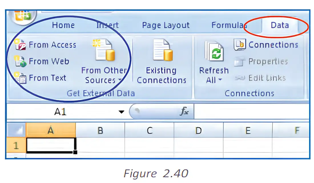
- Import route: In the version described, select Data → Get External Data → From Text, then choose the saved text file.
- Result: Imported data is placed in worksheet rows and columns; the worksheet can then be saved as an Excel data file.
Types and appearance of cell data
Cell content and display
- Labels: Descriptive text, such as names or month names, usually contains letters and is aligned to the left.
- Values: Numeric entries include whole numbers and decimals; whole and decimal values are aligned to the right.
- Decimal display: Excel may omit trailing zeros: for example, `246.70` may display as `246.7`.
- Formulas: Formulas are instructions that tell Excel to perform calculations.
- Dates: Excel may display an entered date in a different format. For example, an entry such as `16/12` may display as `16-Dec`; the formula bar may show `16/12/2008`.
- Date format: Display depends partly on the country-specific format setting.
- Formatting: Cell display, column width and alignment can be changed.
- Data validation: The source names data validation alongside labels, values, dates and formulas, but does not explain it.
Do not assume that a cell’s displayed value exactly matches its entered form: trailing decimal zeros may be hidden, and dates may display in different formats. Excel aligns text labels to the left and numeric values, including dates, to the right; formula results are aligned according to their value type.
How does a CSV file map to spreadsheet rows and columns?
How do labels and numeric values typically align in Excel?
Quick recap
- Data can be copied or imported from text and non-text files.
- In a CSV file, each line becomes a row and commas separate fields into columns.
- The first line can contain column headings; keep later fields in the same order, including blank fields.
- Text labels are usually left-aligned; whole and decimal values are right-aligned.
- Excel may hide trailing decimal zeros and display dates in a different format.
- Formulas instruct Excel to calculate; the source mentions data validation but does not define it.
Data Entry Text Management And Cell Formatting Part III
Data Validation
Data validation — A spreadsheet feature that sets rules for the type or values of data allowed in a cell.
Purpose and benefits
- Accuracy: Restricts invalid entries and helps keep spreadsheet data accurate and consistent.
- Guidance: Input messages tell users what to enter; error alerts respond when an entry breaks a rule.
Creating a Drop-Down List
Uses and examples
- Drop-down list: Offers predefined values and limits entries to the options provided.
- Examples: Department names such as Sales, Finance, R&D, Operations, HR and IT; qualifications such as MBA, PhD, CA, MCA, Architect and MBBS; sex codes Male or Female.
| Method | How it works |
|---|---|
| Delimited list | Type values separated by commas, for example Male, Female. |
| Worksheet cells | Select a row or column of cells containing the list values. |
| Named range | Name a range containing the values and use that name as the source. |
Set up a named-range drop-down list
- Create worksheet headers such as Employee Name, Department, Qualification and Sex Code; enter employee names beneath the first header.
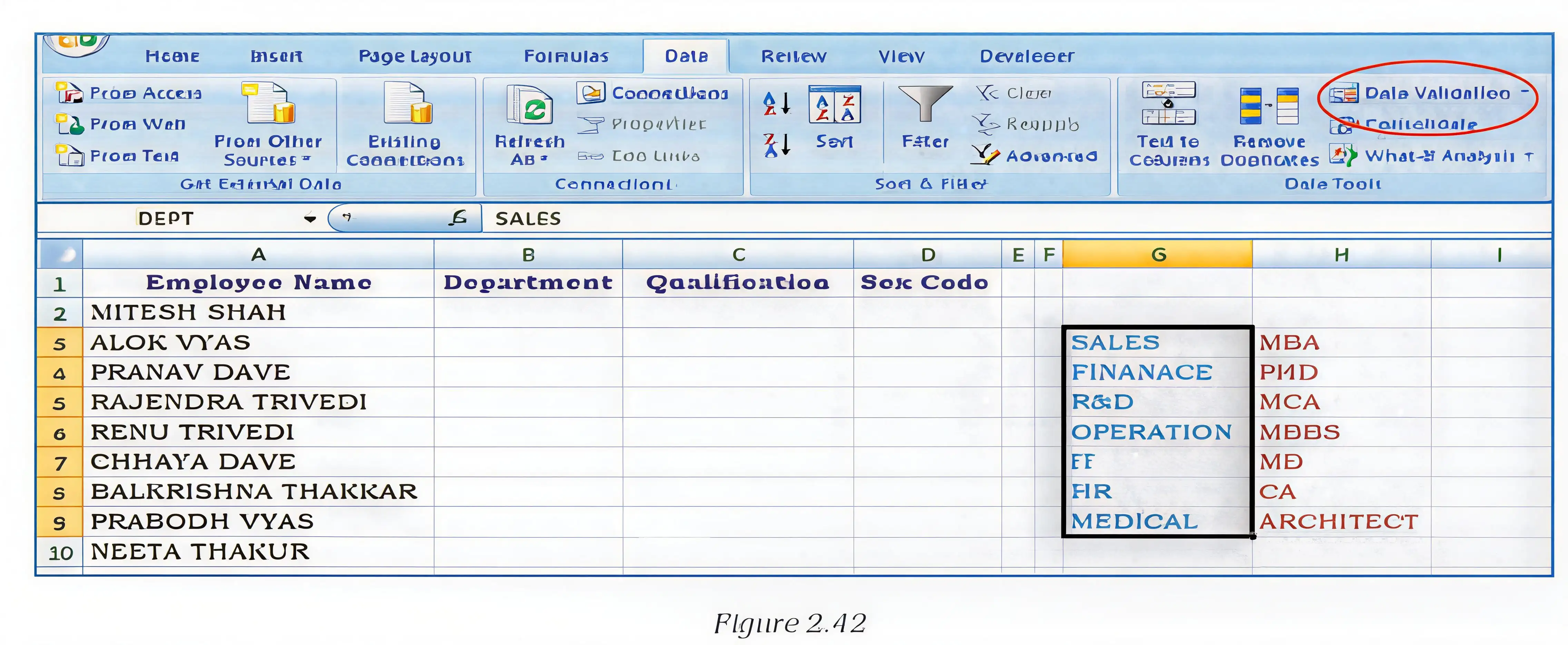
- Enter the department options in a worksheet range, for example G3:G9, then define the range name DEPT using Formula > Define Name.
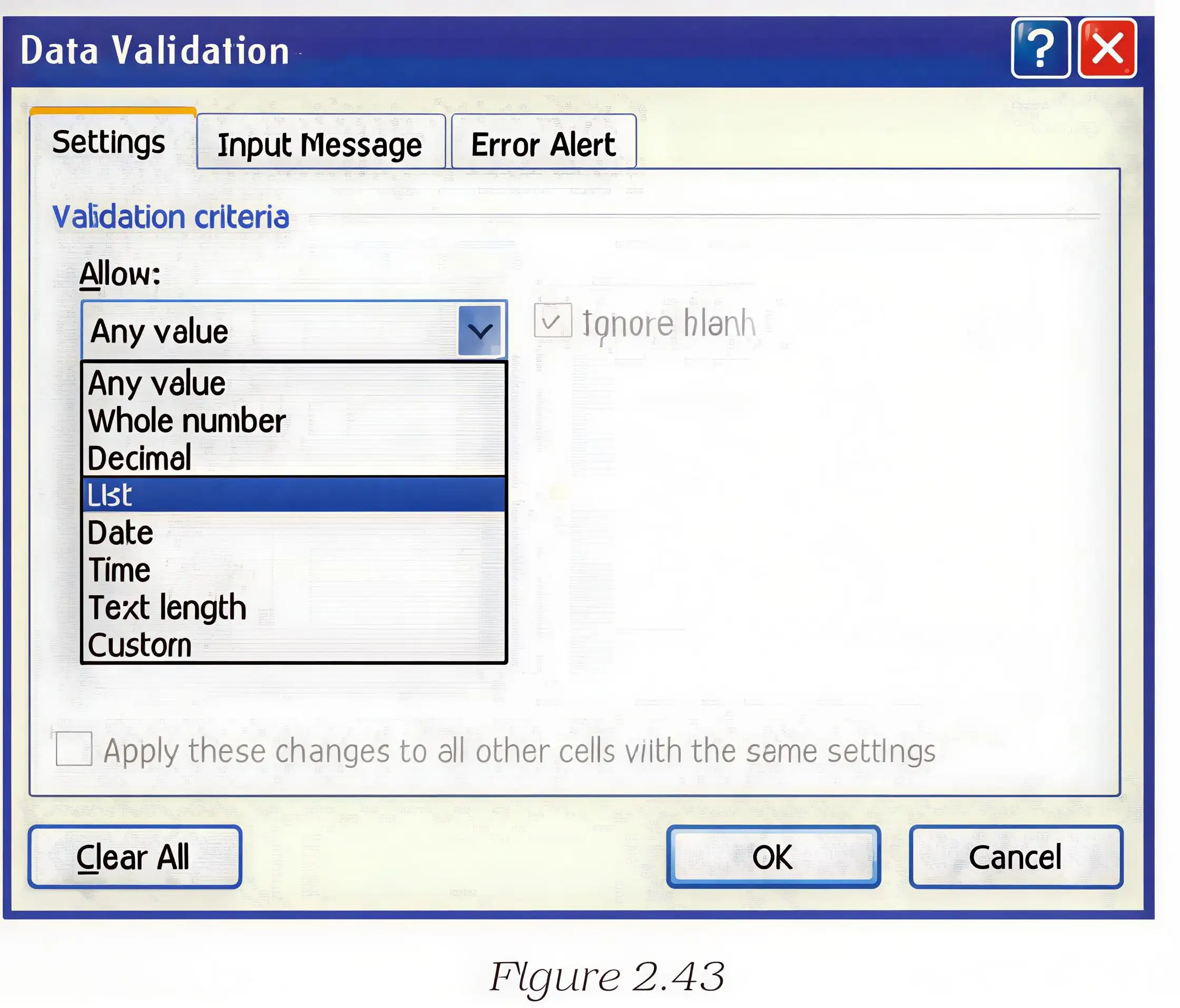
- Select the Department cells to validate, then open Data > Data Validation from the Data Tools group.
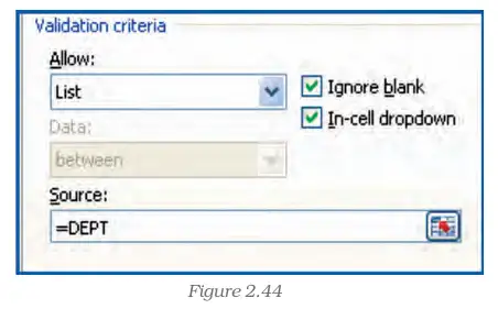
- On the Settings tab, choose List and enter =DEPT in Source; enable Ignore Blank and the in-cell drop-down.
Ignore Blank option
- Effect: As described in this lecture, selecting Ignore Blank means empty or blank values will not be allowed.
Input Messages and Error Alerts
Input message
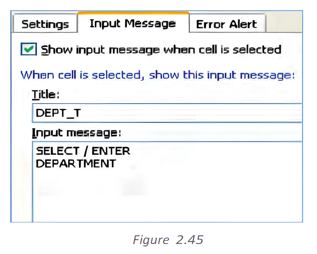
- Purpose: Displays guidance when a validated cell is selected, such as B2 or the range B3:B10.
- Setup: On the Input Message tab, enter a title (for example, DEPT_T) and a short instruction (for example, SELECT/ENTER DEPARTMENT); enable display when the cell is selected.
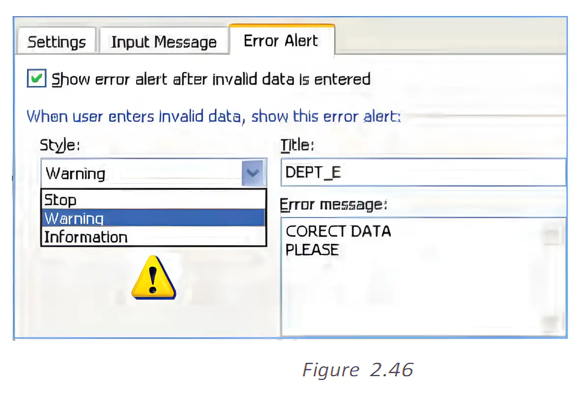
| Style | Effect |
|---|---|
| Stop | Prevents invalid data from being entered. |
| Warning | Shows a warning but does not prevent the invalid entry. |
| Information | Displays an information message and prevents invalid data from being entered. |
Configure an error alert
- Setup: On the Error Alert tab, enable the alert, enter a title and message, then select Information, Warning or Stop according to the required level of control.
Quick recap
- Data validation restricts cell entries to improve accuracy and consistency.
- Drop-down values can come from a comma-separated list, worksheet cells or a named range.
- For a named-range list, select List in Settings and enter the range name as the Source.
- Selecting Ignore Blank means blank values will not be allowed, as described in this lecture.
- Input messages guide users when they select a validated cell.
- Information and Stop prevent invalid entries; Warning displays a warning but allows them.
Data Entry Text Management And Cell Formatting Part IV
Data Validation Using a List
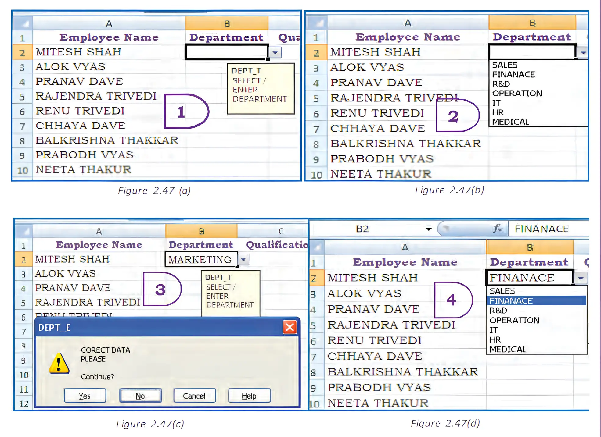
Set up a list
- Select the cells to control and open Data Validation.
- Choose List as the allowed data type.
- Enter the allowed items in the Source box, separated by commas, then set an error alert if needed.
How can a cell be restricted to Male or Female?
- To restrict a Sex Code cell to two entries, choose List and enter the allowed values.
- A valid listed value is accepted; an unlisted or differently capitalised value may be rejected.
Setting Numeric and Text Limits
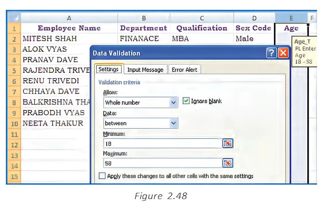
Set a permitted range
- Select the cells and open Data Validation.
- Choose the required type, such as Whole Number or Text Length.
- Select the boundary condition and enter the minimum and/or maximum values.
- Set an error alert to explain rejected entries.
What validation rule allows employee ages from 18 through 58?
- For an employee age cell, choose Whole Number and set the inclusive lower and upper limits.
- An age within the range is accepted; an age below 18 or above 58 is rejected.
Formula-Based Data Validation
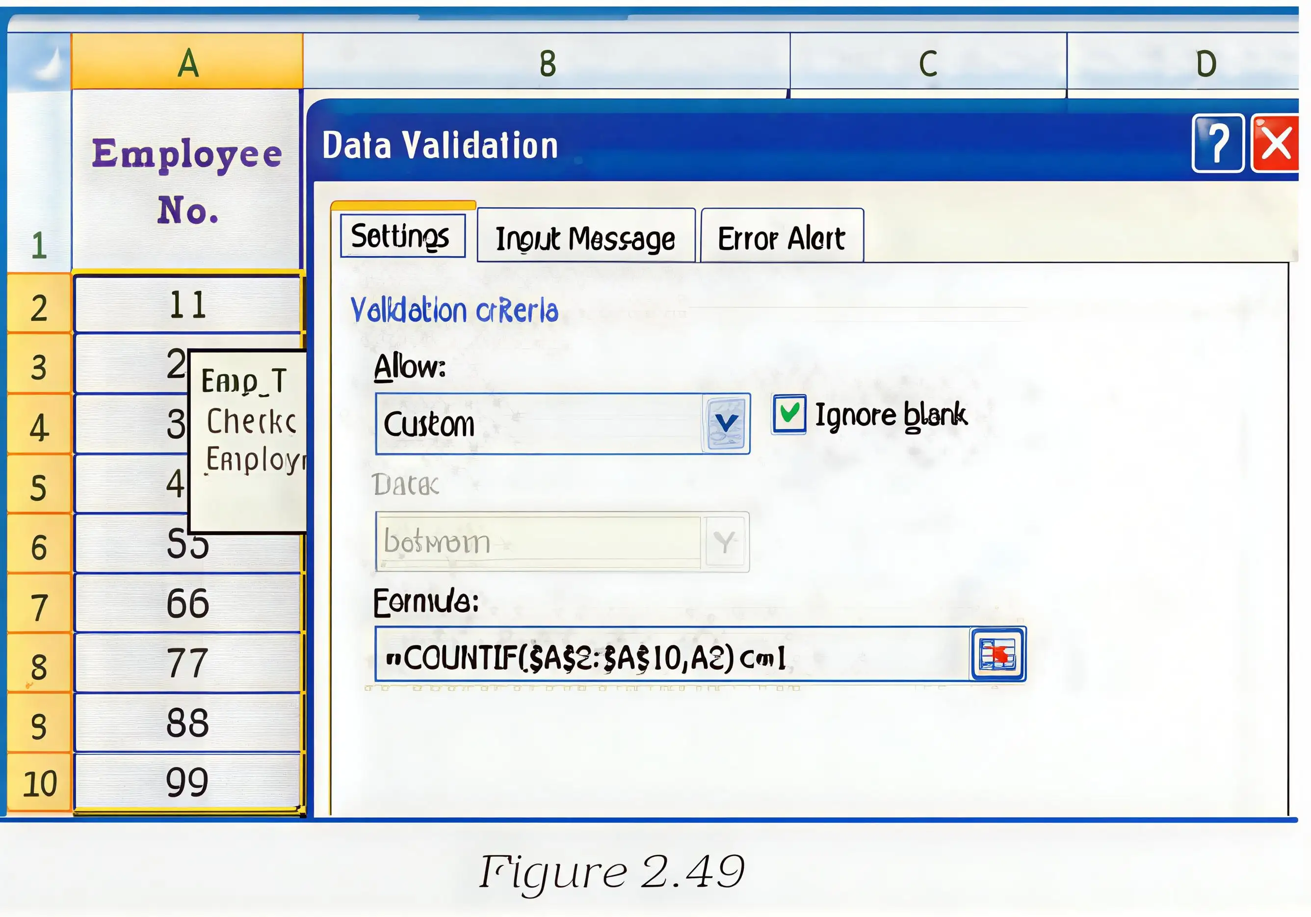
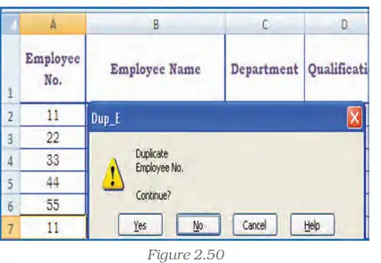
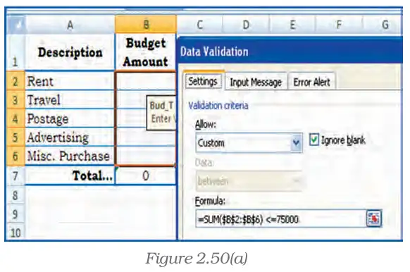
Adjust cell references to match the worksheet. To exclude holidays, also check that the date is absent from a holiday list.
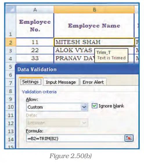
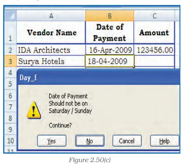
Create a custom validation rule
- Select the cell or range to validate and open Data Validation.
- Choose Custom in the Allow menu.
- Enter a formula that evaluates to TRUE for valid entries and FALSE for invalid entries.
- Configure the error alert so users know why an entry was rejected.
How can duplicate employee numbers be blocked in B2:B100?
- To prevent duplicate codes in B2:B100, count how many times the current entry occurs in the range.
- Allow the entry only when its count is exactly one.
- If the code is already present, the formula returns FALSE and validation blocks the duplicate.
Do not assume a custom formula rejects entries when it returns TRUE: TRUE means the entry is valid. Check that formula references match the validated cells and range.
Write a custom validation formula to prevent extra leading or trailing spaces in cell B2.
Write a validation formula to reject weekend dates entered in A2.
Amounts are in C2:C10 and the budget limit is in F1. Write a formula that prevents the total from exceeding the budget.
Quick recap
- List validation restricts entries to specified values; the list method may be case-sensitive.
- Use Whole Number, Decimal, Date, Time, or Text Length limits to control permitted entries.
- For employee ages, use Whole Number from 18 through 58, or enter a Date of Birth and calculate age.
- Custom validation accepts an entry when its formula evaluates to TRUE and rejects it when FALSE.
- COUNTIF can block duplicate codes, while SUM can enforce a budget ceiling.
- TRIM can detect extra leading or trailing spaces; WEEKDAY can block weekend dates.
Data Entry Text Management And Cell Formatting Part V
Data Forms
Form — A form is a document with a standard structure for capturing, organising and editing information.
Data form — A data form is a dialog box that displays one complete spreadsheet record at a time, making it easier to add, find, change or delete records.
Purpose and use
- Easier entry: Use a data form instead of moving across many columns, especially when all columns cannot fit on the screen.
- Other entry option: Spreadsheet data may also be entered using drop-down lists.
- Best suited to: Simple records where text boxes labelled with column headings are enough; it is not designed for sophisticated custom controls such as list boxes or spin buttons.
Adding the Form Button in Excel 2007
Before opening a data form
- Column headings: Enter all data names in the worksheet’s first row; the form uses these names as field labels.
- Button location: The Form button is not included on the Ribbon by default, so add it to the Quick Access Toolbar.
Add Form to the Quick Access Toolbar
- Click the arrow beside the Quick Access Toolbar, then choose More Commands.
- In “Choose commands from,” select All Commands.
- Select Form in the command list and click Add.
Using the Built-In Data Form
Form features and limits
- Layout: Excel creates a dialog box showing the column headings as labels, each beside a text box for that field.
- Column limit: A data form can display up to 32 columns.
- Record actions: Enter new rows; navigate to or find rows using their contents; update existing rows; and delete rows.
- Formula cells: The form displays a formula’s result, but the formula itself cannot be changed through the form.
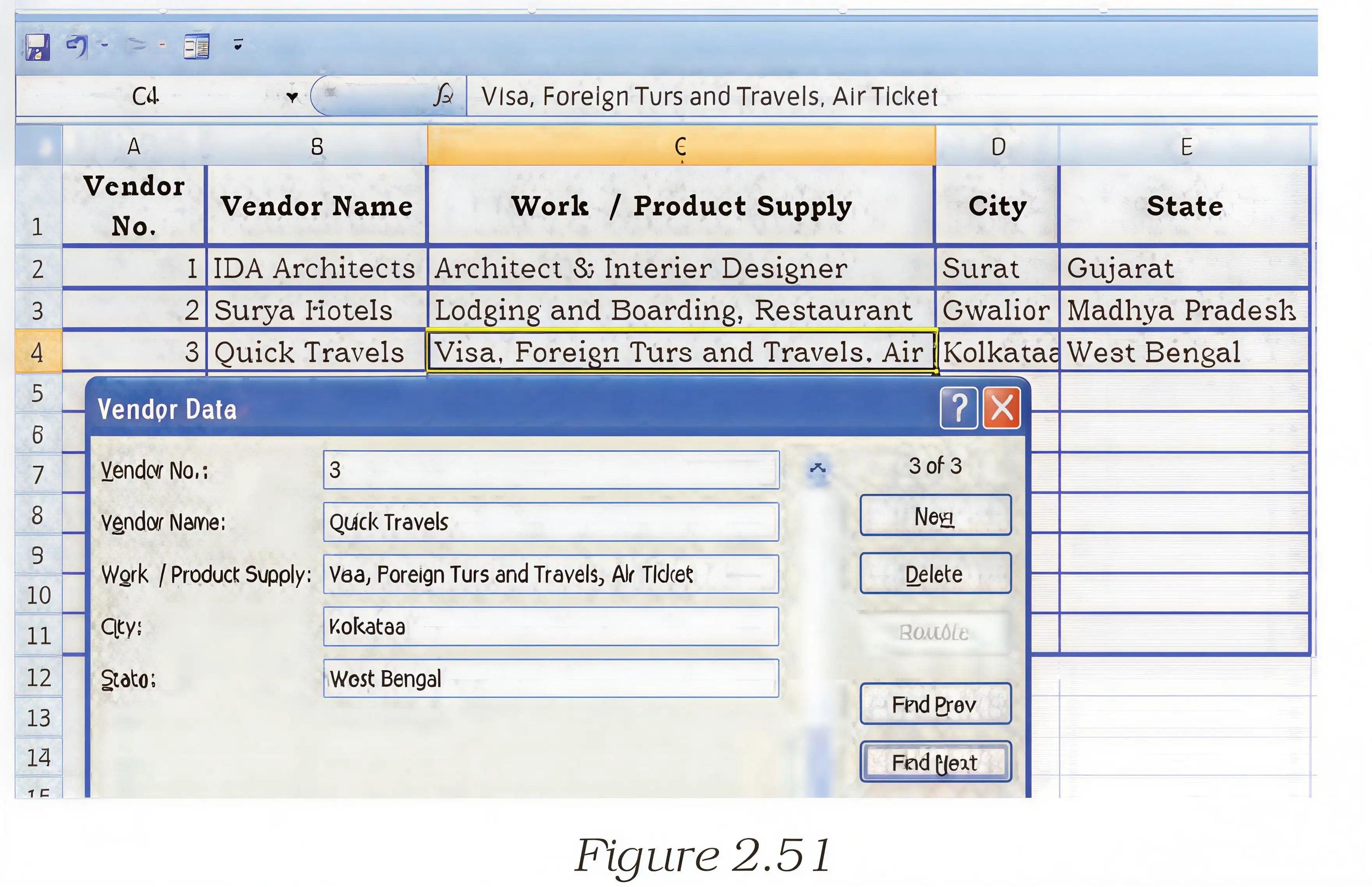
- First row = field names: Data forms use the worksheet’s first-row headings as labels.
- Formula results are viewable, not editable: Change formulas in the worksheet, not through the data form.
Quick recap
- A form uses a standard structure to capture, organise and edit information.
- A data form displays one complete spreadsheet record at a time.
- It helps enter, find, update and delete spreadsheet records.
- Put the column names in the worksheet’s first row before using the form.
- In Excel 2007, add the Form button to the Quick Access Toolbar through More Commands.
- The built-in form supports up to 32 columns and uses labelled text boxes.
- Formula results appear in the form, but formulas cannot be edited there.
Data Formatting Part I
Spreadsheet formatting — Formatting changes how spreadsheet information is displayed so that important data is easier to read and understand.
Number formats
- Number formatting controls how values appear, including currency, percentages, commas, decimal places, dates, times, scientific values and special numbers.
- Automatic recognition Excel may assign a format when a value is entered in a recognizable pattern.
- Currency Entering a value with a currency sign and two decimal places can cause Excel to apply a Currency format.
- Percentage Entering a whole-number percentage followed by % can cause Excel to apply Percentage format.
- Date A recognizable date such as 16-04-2009 or 16 Apr-2009 is treated as a date and displayed in a date format.
- Display vs value Number formatting changes how a value appears; it does not change the underlying value.
| Format | Example display | Purpose |
|---|---|---|
| Currency | Rs. 40 | Shows a currency symbol with a financial value. |
| Percentage | 0.856 displayed as 85.60% | Shows a value as a percentage; decimal places can be set. |
| Date | 16-04-2009 | Displays a date using a recognized date pattern. |
| Special | Phone number or ZIP code | Displays numbers in a format appropriate to a specific country or use. |
Applying number formats
Apply Currency or Percentage format
- Select the cell or range to format.
- Open the Format Cells dialog from the Home tab’s Number options.
- On the Number tab, choose the required category, such as Currency or Percentage.
- Set options such as currency symbol, negative-value style or number of decimal places.
- Click OK to apply the selected format.
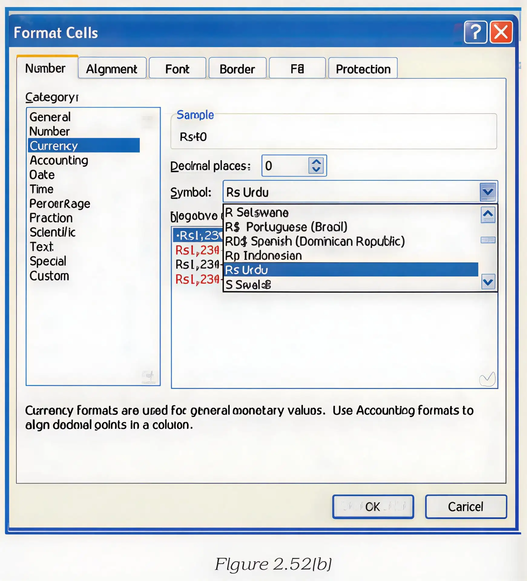
How can ranges B4:E7 and H4:H8 be formatted as Currency with no decimals and Percentage with two decimals, respectively?
- To format B4:E7 as Currency with zero decimal places, select the range B4:E7.
- Open Format Cells and choose Currency on the Number tab.
- Set decimal places to 0 and choose the required negative-number style.
- Click OK; the selected values display as currency rounded to whole units, for example Rs. 40.
- To show H4:H8 as percentages to two decimal places, repeat the process using Percentage and set decimal places to 2; 0.856 displays as 85.60%.
Do not confuse a displayed percentage with the stored value: formatting 0.856 as Percentage displays 85.60%, but the underlying value remains 0.856.
Special number formats
- Use Special formats are designed for numbers such as telephone numbers, ZIP codes and Social Security numbers.
- Set format In Format Cells, choose Special, then select the suitable format from the Locale list for the relevant country.
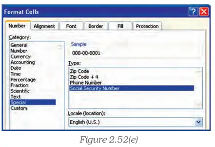
Cell colours and patterns
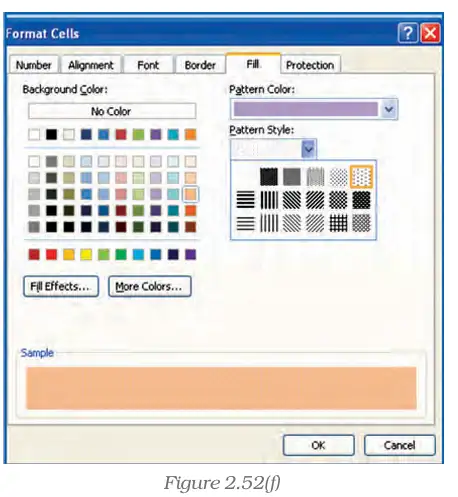
Change cell fill
- Select the cell or range to format.
- Open Format Cells from the Home tab’s Number options and choose the Fill tab.
- Choose a background colour, pattern colour and pattern style as needed.
- Click OK to apply the fill to the selected cells.
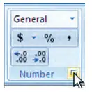
Ribbon number-formatting controls
- Comma Style Adds comma separators to large numbers to make them easier to read; it may also display two decimal places.
- Decrease Decimal Removes one displayed decimal place each time the button is clicked.
- Increase Decimal Adds displayed decimal places; click as often as required.
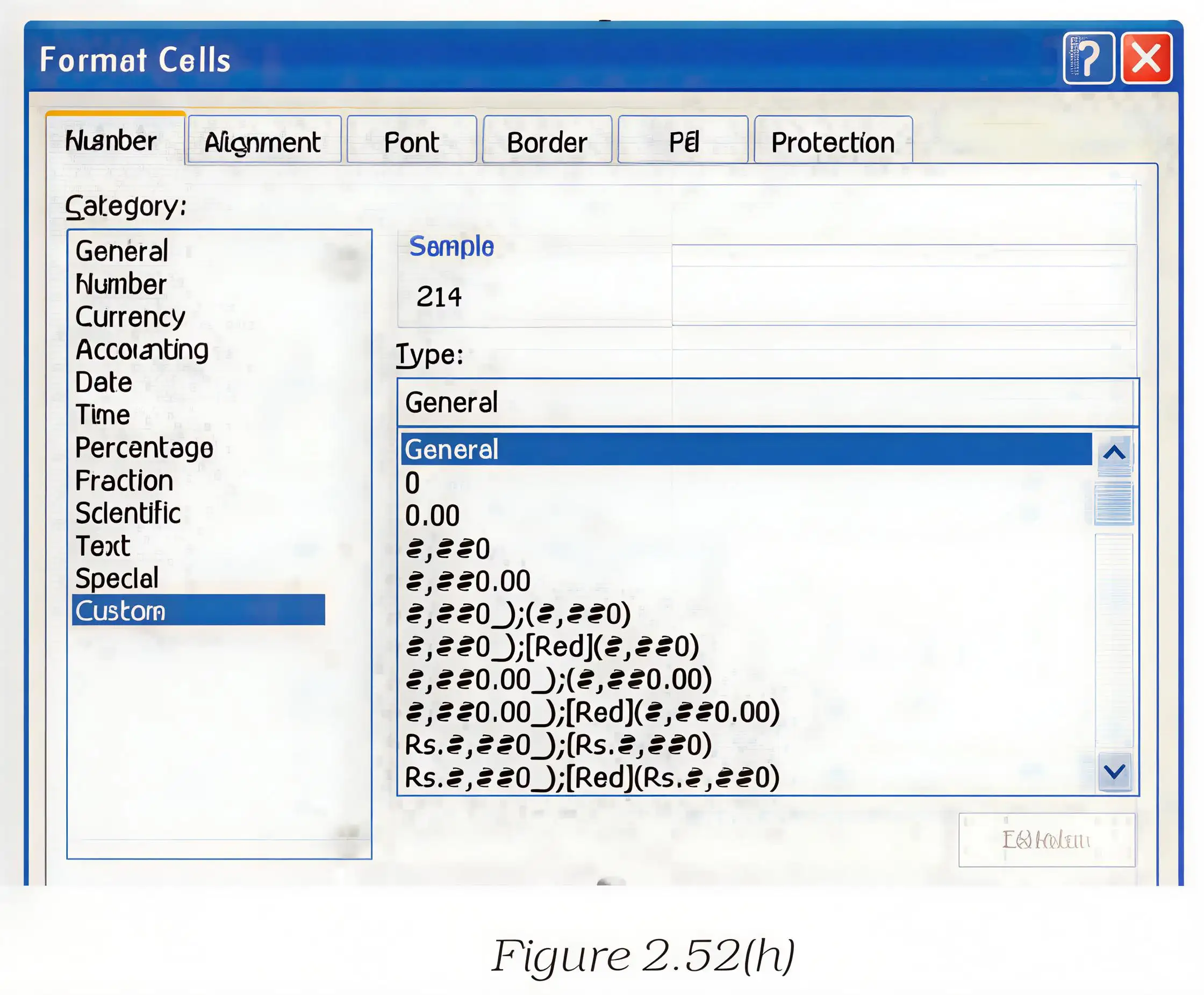
Custom formats and checking existing formats
- Custom format In Format Cells, choose Custom, select an existing format and add characters or remove unwanted ones to create the desired display.
- Inspect or change Right-click the cell, cells or column and choose Format Cells; identify the current category or select a suitable new or custom format.
How do you format a selected range as Currency with zero decimal places?
Which format is suitable for telephone numbers, and how is it selected?
A cell contains 1.2636. What will it display after applying Percentage format with two decimal places?
How would you display a number with a comma separator and remove its displayed decimal places?
Quick recap
- Number formatting controls the display of currency, percentages, dates, decimals, commas and special numbers.
- Format Cells lets you choose a category and set options such as decimal places and negative-value style.
- Percentage formatting changes how a value is displayed, not its stored value.
- Fill formatting offers background colours and cell patterns.
- Ribbon controls provide Comma Style and quick decimal-place adjustments.
- Custom formats can be edited, and existing formats can be checked through Format Cells.
Data Formatting Part II
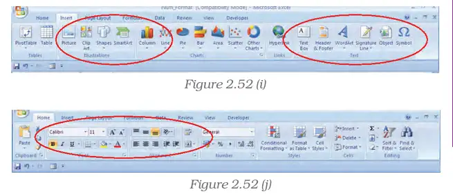
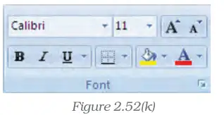
Text Formatting
Cell Borders
Custom Cell Border Styles
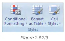
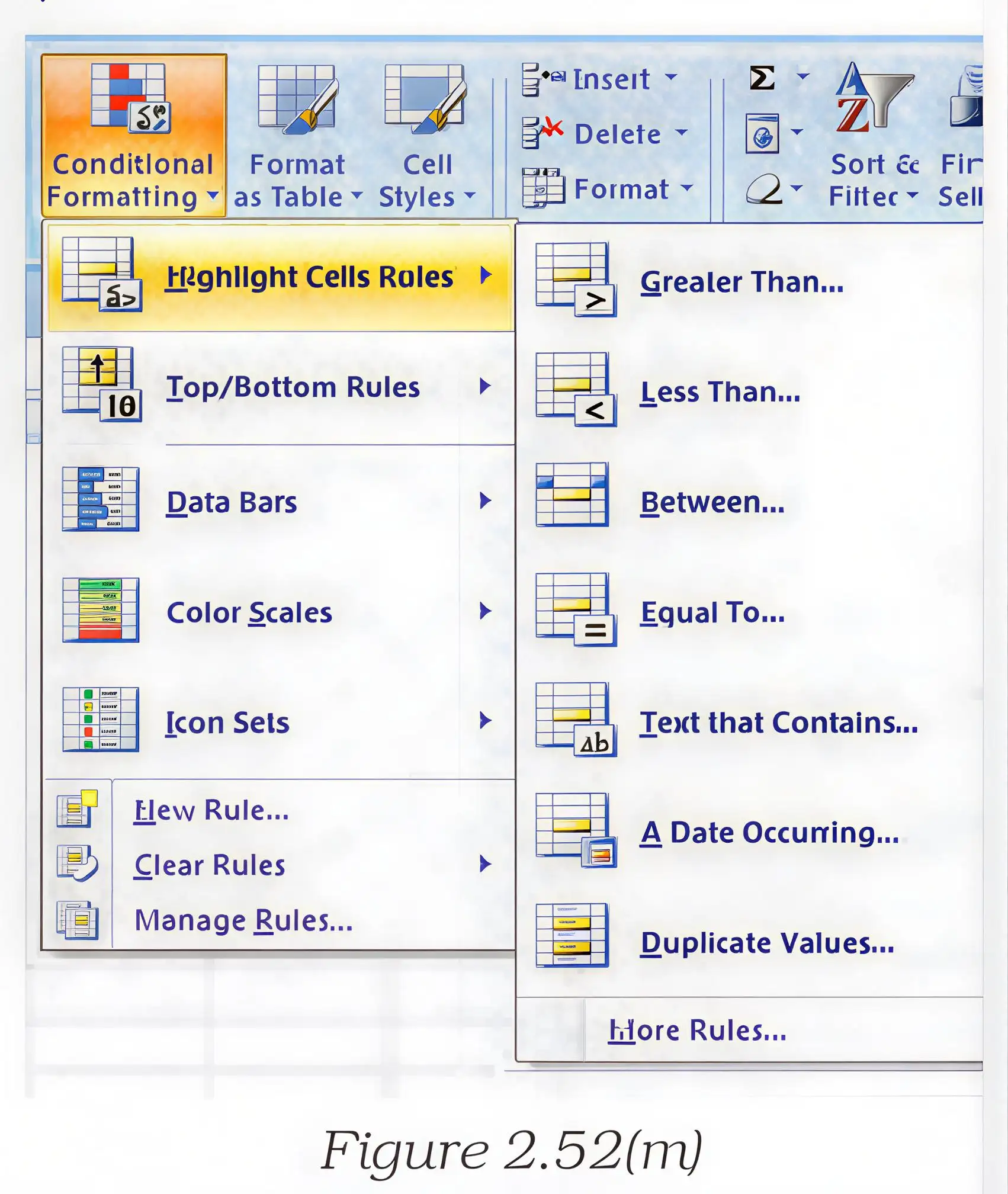
Conditional Formatting
Quick recap
- Text formatting improves readability and presentation through font, size, alignment, colour and cell merging.
- Use the Home-tab Font group to change text appearance.
- The Borders menu applies, changes or removes borders; the button reapplies the most recently used style.
- Custom cell styles can save border settings for reuse on selected cells.
- Conditional formatting makes data easier to analyse by formatting cells according to criteria.
- Data bars, colour scales and icon sets can help reveal values, exceptions and trends.
Data Formatting Part III
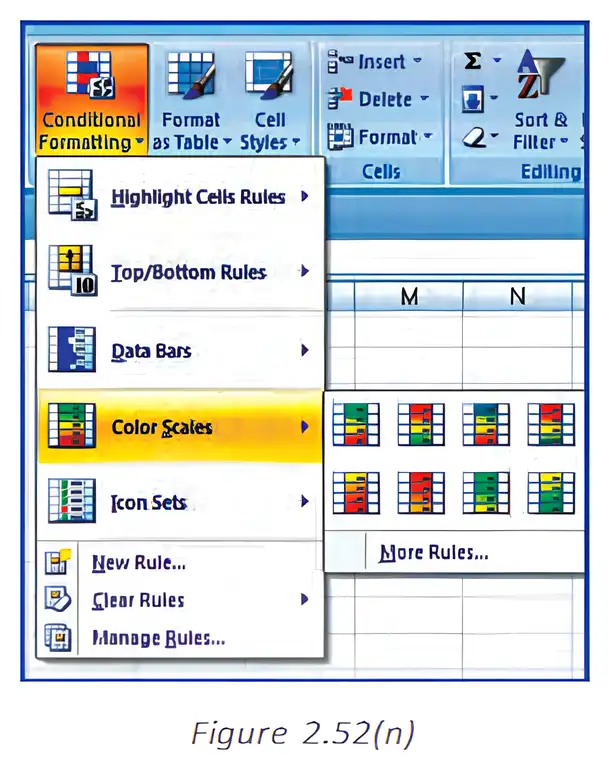
Colour Scales
Creating a Three-Colour Scale
| Type | How it works / requirement |
|---|---|
| Lowest Value / Highest Value | Uses the lowest and highest values in the range; no Minimum or Maximum value needs to be entered. |
| Number | Uses specified numeric Minimum and Maximum values. |
| Per cent | Enter values from 0 to 100 without a percent sign. Use when the distribution of values is proportional and you want to visualise values proportionally. |
| Percentile | Enter percentile values from 0 to 100. Useful for highlighting groups of high or extreme values that may skew the visualisation. |
| Formula | The formula must start with an equal sign and return a number, date or time. Test it in the worksheet and ensure it does not return an error. |
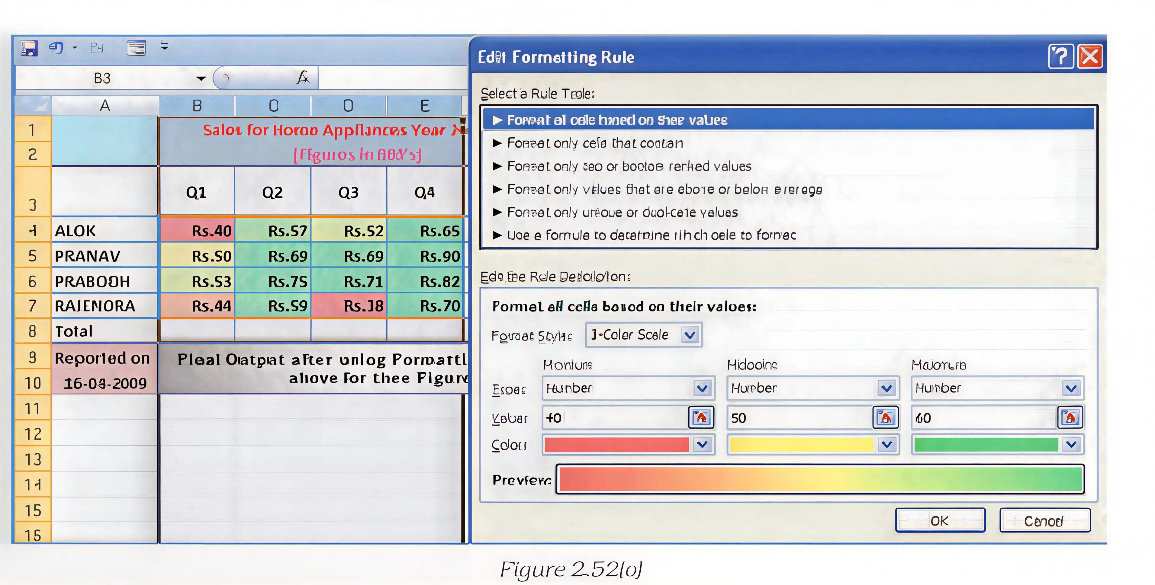
How do you apply a three-colour scale to a selected range?
- Select the required cell range and open Manage Rules from Conditional Formatting.
- Click New Rule, choose Format all cells based on their values, and select 3-Colour Scale.
- Choose the required Minimum and Maximum types and values, then confirm the rule.
Changing Text Alignment
Set Cell Alignment
- Select the cell range.
- Open the Alignment options from the Home tab and display the Format Cells dialog.
- On the Alignment tab, select the required horizontal and vertical alignment.
- Adjust text orientation or cell text-fit options if required, then click OK.
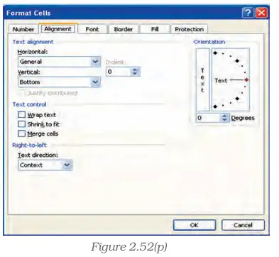
How can you centre data horizontally and vertically in selected cells?
- Select the cells whose data needs alignment.
- Open Format Cells and select the Alignment tab.
- Choose the required horizontal and vertical alignment, then click OK.
A selected range contains formula errors, so its colour scale does not apply throughout. What should you do?
What values are allowed for a Percentile type, and when is it useful?
Quick recap
- Colour scales compare values through graduated colours; red may indicate lower values and green higher values.
- Use Home → Conditional Formatting → Colour Scales to apply a two-colour scale.
- Create or edit a three-colour rule through Manage Rules; choose Format all cells based on their values and 3-Colour Scale.
- Minimum and Maximum types include Lowest/Highest Value, Number, Per cent, Percentile and Formula, each with its own input requirements.
- Formula errors can prevent a colour scale applying to a whole range; use IS or IFERROR to return a non-error value.
- Cell alignment settings control horizontal and vertical position, orientation and text fit; chart elements also offer direction, autofit, margins and columns.
Data Formatting Part IV
Merging and Splitting Cells
Merge or split cells
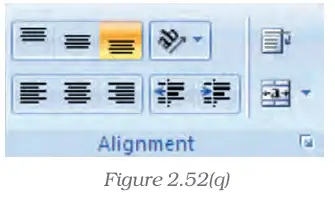
- Select two or more adjacent cells to merge.
- On Home > Alignment, click Merge and Centre, or use its arrow to choose Merge Across or Merge Cells.
- To split cells, select the merged cell and click Merge and Centre again.
How can a heading be centred across cells A1:D1 and then unmerged?
- To centre a heading over cells A1:D1, select A1:D1 and click Merge and Centre.
- The range becomes one cell, referenced as A1, with the heading centred.
- To restore the four cells, select the merged cell and click Merge and Centre again; the text returns to A1.
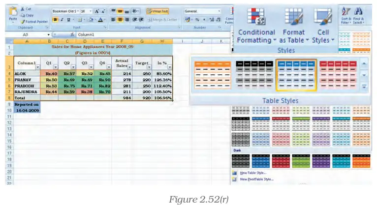
Formatting a Table
How do you quickly apply a predefined style to a selected data range?
- Select the sales-data range that you want to format as a table.
- Choose Home > Format as Table and select a style from Light, Medium or Dark.
- The chosen table style formats the selected data; table-element options can emphasize headings, totals, columns or alternating bands.
Using the NOW Function
What does NOW() return, and what does the decimal part of its serial value represent?
- Enter =NOW() in a cell formatted as General.
- Excel returns the current date-and-time serial value and displays it as a date and time.
- In the serial value, the integer part represents the date and the decimal part represents the time.
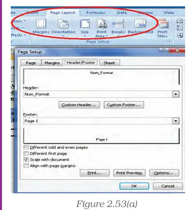
Adding Headers and Footers
Add or change worksheet header or footer text
- Select the worksheet and choose Insert > Text > Header and Footer.
- Click the left, centre or right header/footer text box at the top or bottom of the page.
- Type new text, or select and replace existing text.
How can you place a title at the top centre of printed worksheet pages?
- Select the worksheet and open Insert > Header and Footer.
- Click the centre header box and enter the spreadsheet title.
- The title will appear in the header when the worksheet is printed.
Format Painter
How can newly added cells be made to match the formatting of existing cells?
- Select a cell that has the formatting you want to copy.
- Use Format Painter and apply it to the newly added cells.
- The target cells take on the source formatting.
AutoFormat
What is the purpose of AutoFormat?
- Choose an AutoFormat style from the available Excel 2007 options.
- The style applies its combined formatting features to the spreadsheet.
Quick recap
- Merge: A merged range uses the upper-left cell’s reference; Merge Across works across selected rows.
- Split: Unmerging restores the cells and places the content in the upper-left cell.
- Table styles: Choose Light, Medium or Dark styles; options can format headers, totals, columns and bands.
- NOW(): Returns the current date-and-time serial value; its integer and decimal parts represent date and time.
- Serial dates: January 1, 1900 = 1; January 1, 2008 = 39448; 0.5 represents noon.
- Page and cell formatting: Headers/footers add print information, Format Painter copies formatting, and AutoFormat applies presets.
Output Reports
Printing Worksheets and Workbooks
Output report — A printed or file-based copy of spreadsheet data, worksheets, workbooks, charts, or PivotTables.
| Print option | Purpose |
|---|---|
| Worksheets or workbooks | Print all or selected parts; print one or several worksheets or workbooks. |
| Tables, charts, and PivotTables | Print spreadsheet tables and visual or summary reports. |
| Workbook to a file | Save the workbook as a print output instead of sending it directly to a printer; useful when printing later on another printer. |
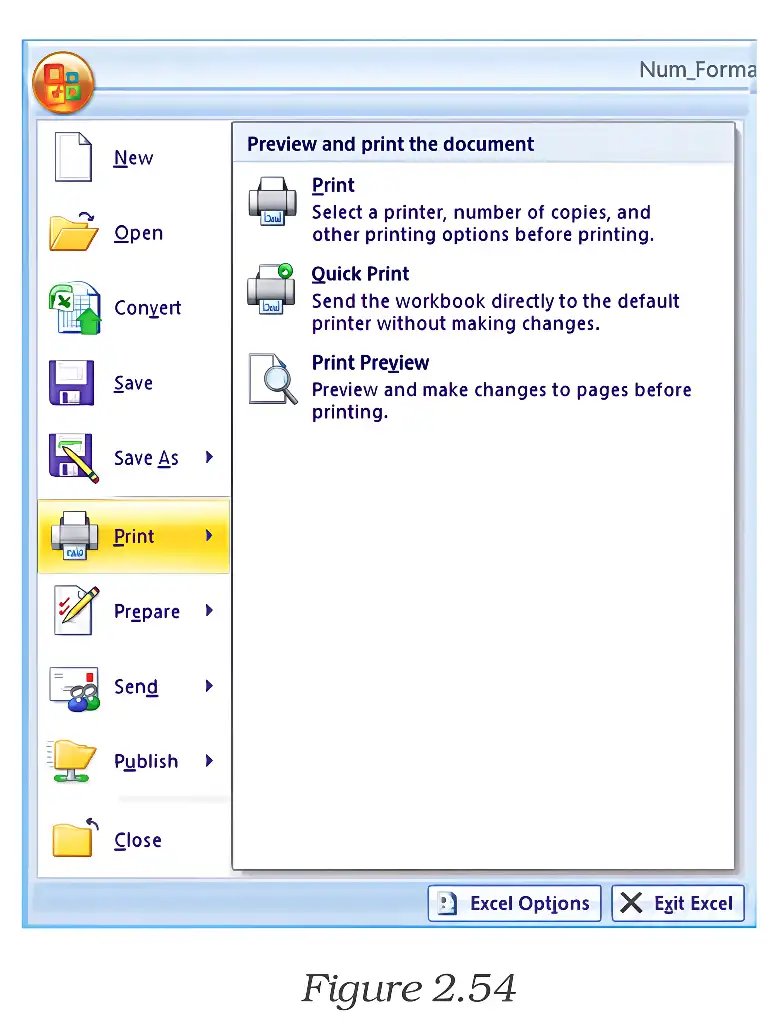
| Quick Print / Print Preview | Quick Print sends the output directly to print; Print Preview lets you check it before printing. |
Defining the Print Area
Print area — The selected worksheet cell range that Excel is set to print; by default, Excel prints all data on the current worksheet.
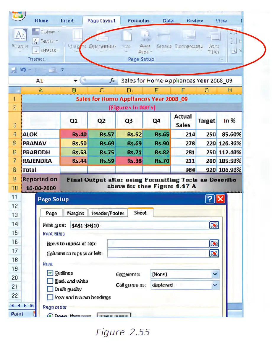
Set a print area through Page Setup
- Open the Page Layout tab and choose Page Setup.
- In the Page Setup dialog box, open the Sheet tab.
- Enter the cell range in the Print Area box, or use Collapse Dialog to select the range and Restore Dialog to return.
- Click OK to define the print area.
Set, expand, or clear a print area
- Select the cells to print, such as A1:H10.
- Choose Page Layout → Print Area → Set Print Area.
- To include additional cells, select them and choose Print Area → Add to Print Area; repeat as needed.
- To remove the defined area, choose Print Area → Clear Print Area.
- Print-area setting: It remains active until it is cleared or replaced.
- Add to Print Area: Adds selected cells to an existing print area.
Printing Selected Cell Ranges
Print a selected range
- Select the cell range, or choose a named range from the Name Box list.
- Open Print using the Office Button menu or press Ctrl+P.
- In the Print what section, choose Selection, then confirm to print.
Print multiple non-contiguous ranges
- Select the first cell range.
- Hold Ctrl while selecting each additional range.
- Open Print using the Office Button menu or press Ctrl+P.
- Choose Selection in the Print what section and print; each selected range prints on a separate page.
Do not confuse a defined print area with printing a temporary selection: a print area stays set until changed or cleared, while Selection prints the ranges currently selected.
Quick recap
- Excel can print entire or partial worksheets and workbooks, multiple sheets or workbooks, tables, charts, and PivotTables.
- Quick Print sends output directly to print; Print Preview checks the layout first.
- By default, Excel prints all data on the current worksheet; define a print area for a specific range.
- A print area can be set through Page Setup or Page Layout → Print Area and expanded or cleared there.
- Select a range and choose Selection in the Print dialog to print only that range.
- Use Ctrl while selecting ranges to print multiple non-contiguous ranges; each prints on a separate page.
Preparation Of Reports Using Pivot Table Part I
Pivot Table Reports and Data Tables
- Data tables: What-if data tables show how changing one or two input values affects a formula’s result.
- PivotTable reports: These summarise and arrange data from a list or table, allowing fields to be grouped and rearranged for different views.
- Use: Both tools help analyse data and present results in a useful report format.
One-Variable Data Table
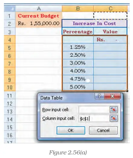
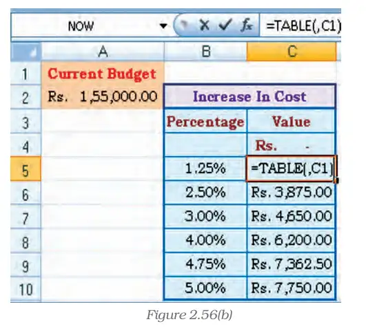
Enter this spreadsheet formula in C4; each percentage is substituted into C1.
Set Up a Column-Oriented One-Variable Table
- Enter the formula `=A2*C1` in C4 and list the percentages in B5:B10.
- Select B4:C10, then choose Data > What-if Analysis > Data Table.
- Leave Row input cell blank and enter `1` as the Column input cell; click OK.
Two-Variable Data Table
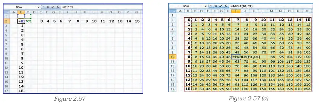
Enter this spreadsheet formula in B2; the two input lists supply values to B1 and C1.
Set Up a Two-Variable Data Table
- Enter `=B1*C1` in B2.
- Enter one list down B3:B17 and the other across C3:Q3.
- Select B2:Q17 and choose Data > What-if Analysis > Data Table.
- Set Row input cell to `1` for the top-row values and Column input cell to `1` for the first-column values; click OK.
What is the increase on a current budget of Rs. 1,55,000 when costs rise by 1.25%?
- A current budget is Rs. 1,55,000 and the cost-increase percentage is 1.25%.
- Substitute the percentage into C1 and multiply by the budget using `=A2*C1`.
- The resulting budget increase is Rs. 1,937.50.
For percentages listed down B5:B10, how should the one-variable budget table be set up?
For a multiplication table with values across C3:Q3 and down B3:B17, which input cells should be assigned?
Do not swap the two-variable input settings: values across the top row map to Row input cell `1`, while values down the first column map to Column input cell `1`.
Quick recap
- Pivot Table reports organise list data into readable reports using fields, details, calculations and groups.
- A one-variable data table substitutes a series of values into one input cell; values can be arranged in a row or column.
- For the budget table, enter `=A2*C1` and use `1` as the Column input cell for percentages listed vertically.
- A two-variable data table uses one formula and two input lists mapped to two distinct input cells.
- With values across C3:Q3 and down B3:B17, use `1` as Row input cell and `1` as Column input cell.
Preparation Of Reports Using Pivot Table Part II
Pivot Tables
Use this to compare actual consumption with the fixed quota.
Creating and arranging a PivotTable
Create and set up the report
- Select the complete source data range, .
- On the Insert tab, choose PivotTable in the Tables group to open the report-creation options.
- Choose the data location and select Existing Worksheet; enter a destination such as .
- Click OK to create a blank PivotTable and display the field list.
- Drag fields into the report areas: Day to Report Filter, Vegetable to Column Labels, City to Row Labels, and Actual to Values.
- Use Sum of Actual to aggregate consumption. To change the view, rearrange the fields; for example, place City and then Vegetable in Row Labels and leave Column Labels empty.
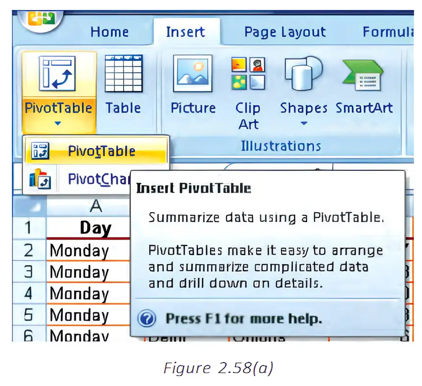
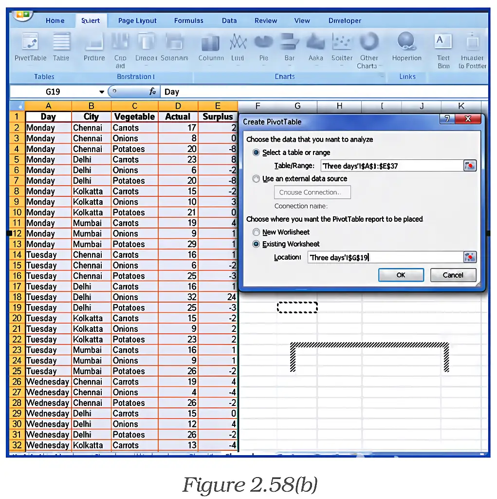
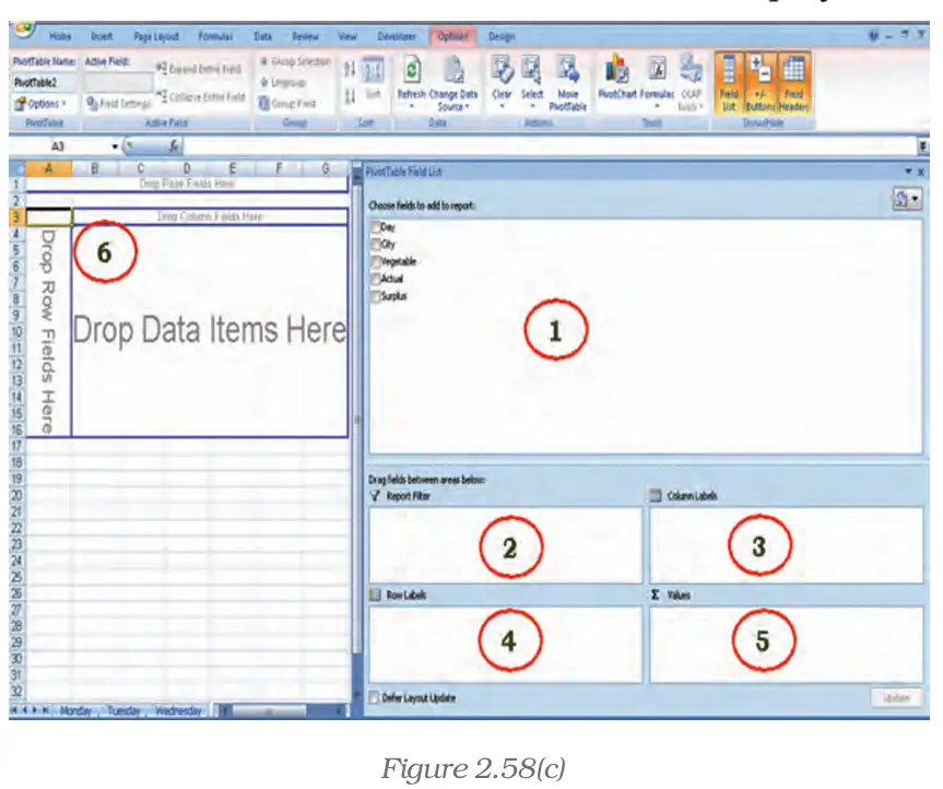
Prepare a report of actual vegetable consumption by city and vegetable, with Day as a filter.
- Select the consumption data for the three vegetables, four cities and three days: .
- Insert a PivotTable and choose Existing Worksheet, placing it at .
- Set Day as Report Filter, Vegetable as Column Labels, City as Row Labels and Actual as Values, summarized by Sum.
- The resulting report shows summed actual consumption by city and vegetable, and allows the user to filter by day.
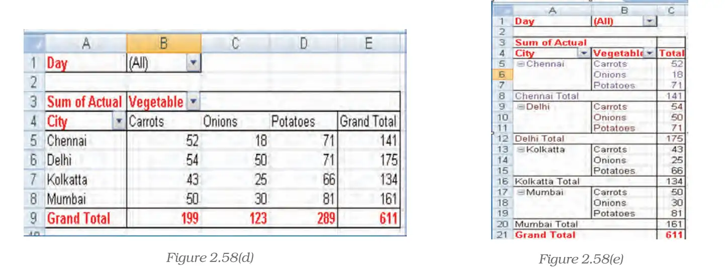
Advantages and uses of PivotTable reports
- Summarize: Query large datasets, aggregate numerical data, calculate subtotals and summarize by categories or subcategories.
- Analyse: Create custom calculations and formulas, and compare related totals or several facts across a long list of figures.
- Expand or collapse: Move between detailed data and summary levels to focus on information of interest.
- Rearrange: Pivot rows into columns or columns into rows to view different summaries of the same source data.
- Filter and organize: Filter, sort, group and conditionally format useful subsets of data.
- Present: Produce concise, attractive and annotated reports for on-screen use or printing.
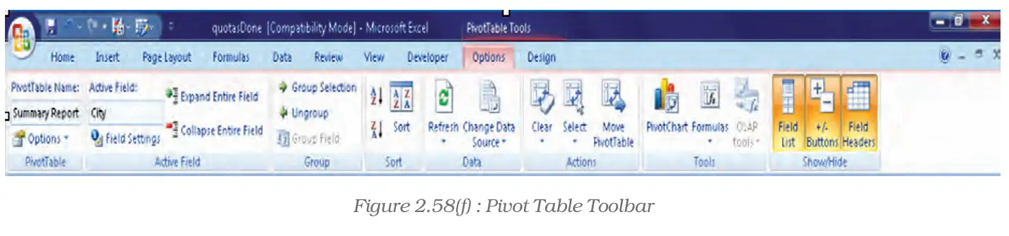
What report layout results from placing City and then Vegetable in Row Labels, with no field in Column Labels?
Which report areas summarize actual consumption by city while allowing one day to be viewed at a time?
Quick recap
- A PivotTable interactively summarizes large amounts of spreadsheet data.
- Report Filter, Column Labels, Row Labels and Values determine the report layout.
- The example summarizes Sum of Actual by city and vegetable, with Day as a filter.
- Rearranging or filtering fields creates different views of the same source data.
- PivotTables support aggregation, subtotals, sorting, grouping and comparisons.
- Surplus is actual consumption minus quota: .
Common Errors (Messages) In Spreadsheet Part I
Checking and marking formula errors
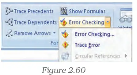
Correcting common error values
- Error checking: Excel can mark possible formula errors and provide an Error Checking tool to review them.
- Diagnosis: Identify the error value and check the formula, its references and the data used in its arguments.
- Correction: Correct the cause of the error or adjust the formula so it handles the relevant conditions appropriately.
The ##### display
Do not assume ##### always means a formula is wrong: first check column width and number format, then check for a negative date or time.
The #DIV/0! error
For a calculation using cells A5 and B5, return a blank result if B5 is zero.
How can a formula avoid displaying #DIV/0! when B5 is zero?
- Suppose A5 contains the amount and B5 contains zero; the direct division formula produces a division-by-zero error.
- Check whether B5 is zero before carrying out the division.
- The formula returns a blank string when B5 is zero; otherwise it calculates A5 divided by B5.
The #N/A error
- Meaning: #N/A appears when a value required by a formula or function is unavailable.
- Common causes: A lookup may use an inappropriate value or an unsorted table; required data may also be missing.
- Check: Verify the lookup value, table arrangement and function arguments.
The #NAME? error
A cell displays #####. Give two possible causes and one correction for each.
A formula divides A5 by B5, and B5 is blank. Why does an error appear, and how can it be prevented?
A lookup formula returns #N/A. Name two possible causes.
Quick recap
- Background checking marks possible formula errors; use Error Checking to review or ignore them.
- ##### usually indicates insufficient column width; it may also signal a negative date/time.
- #DIV/0! results from a zero or blank divisor; correct the divisor or test it with IF.
- #N/A means a required value is unavailable; check data, lookup arguments, sorting and array dimensions.
- #NAME? means Excel does not recognise formula text; a missing required add-in can be the cause.
Common Errors (Messages) In Spreadsheet Part II
#NULL! Error
- Meaning: #NULL! occurs when a formula specifies the intersection of two ranges that do not intersect.
- Range operators: Use a colon for a continuous range, such as A1:A10, and a comma to combine separate ranges.
- Check: Review the formula’s references and range operators to ensure they describe the intended cells.
#NUM! Error
- Meaning: #NUM! indicates an invalid numeric value or an unsuccessful numerical calculation.
- Common causes: A function may receive an unacceptable numeric argument, or an iterative function such as RATE may fail to find a result.
- Correction: Check the arguments and, for an iterative function, try a different starting estimate.
#REF! Error
- Meaning: #REF! indicates that a formula contains an invalid cell reference.
- Common cause: Deleting referenced cells or pasting moved cells over them can invalidate formulas.
- Correction: Restore the affected cells if possible, or edit the formula to use a valid reference.
#VALUE! Error
Why does return #VALUE! in this case, and how can it be fixed?
- A5 contains a number and A6 contains the text “Not available.” The formula adds both cells.
- The text is not a valid numeric operand, so the formula returns #VALUE!.
- Replace the invalid text with a number, or change the formula to use valid numeric cells.
A formula uses , but the ranges do not intersect. What error may appear, and how should the formula be corrected to sum both ranges?
A formula returns #REF! immediately after cells it referred to were deleted. Give one way to correct the problem.
Quick recap
- #NULL! usually signals an incorrect intersection; use a colon for a continuous range and a comma for separate ranges.
- #NUM! indicates an invalid numeric value, an unsuccessful iterative function, or a number outside Excel's range.
- #REF! means a formula's cell reference is invalid, often because cells were deleted or overwritten.
- #VALUE! means a formula has received an argument or operand of the wrong type.
- Array formulas in legacy Excel are confirmed with Ctrl+Shift+Enter when required.
Summary
Spreadsheet Structure and Cells
- Worksheet: Spreadsheet information is organised in a grid of horizontal rows and vertical columns.
- Cell: The intersection of a row and column forms a cell, identified by its column letter and row number, such as B4.
- Workbook: A workbook can contain multiple worksheets, which provide separate grids within one file.
Formulas, Cell References and Ranges
A reference uses followed by a row number and followed by a column number. A relative row or column number is enclosed in square brackets; some spreadsheets offer this style as a compatibility option.
Cell range — A cell range is a group of cells specified by its starting and ending references, such as .
Function — A function is a named instruction that processes the argument or arguments supplied in brackets and returns a result.
Use the SUM function to add all cells from the first reference through the last reference.
What result does the formula produce?
- Suppose cells , and contain , and . Enter the SUM formula in another cell.
- The formula adds the three values in the range.
Formatting a Spreadsheet
- Purpose: Formatting makes spreadsheet information easier to read and understand.
- Options: Number, text and cell formatting can change how values and labels are displayed.
- Display: Formatting changes a cell’s appearance without changing the value stored in it.
Printing a Spreadsheet
- Print options: Excel can print a whole or partial worksheet, selected ranges, multiple sheets or workbooks, and charts or PivotTable reports.
- Print area: Define the cells to print using the Page Setup dialog box or the Print Area command; the defined area remains until cleared or replaced.
- Preview: Use Print Preview to check the output before printing, or choose Quick Print to print directly.
Saving a Spreadsheet
Cells , and contain , and . What does return?
When a formula is copied to another cell, which parts adjust in , and ?
Quick recap
- A spreadsheet uses rows, columns and cells; a workbook can contain multiple named sheets.
- Cells may hold values, formulas, functions or nothing; formulas and functions conventionally begin with .
- References may be relative, absolute or mixed; a dollar sign marks the part that stays fixed when copied.
- A range such as identifies a group of cells; SUM adds the values in that range.
- Formatting changes how contents appear, not the underlying cell contents.
- Page setup controls print orientation; save work regularly and specify a destination and file name.
Formula sheet
Accountancy — ALL CHAPTERS
1
Accounting for Share Capital
2
Issue and Redemption of Debentures
3
Financial Statements of a Company
4
Analysis of Financial Statements
5
Accounting Ratios
6
Cash Flow Statement
1
Overview Of Computerised Accounting System
2
Spreadsheet
3
Use Of Spreadsheet In Business Applications
4
Graphs And Charts For Business Data
1
Accounting for Partnership: Basic Concepts
2
Reconstitution of a Partnership Firm –Admission of a Partner
3
Reconstitution of a Partnership Firm –Retirement/Death of a Partner
4
Dissolution of Partnership Firm