Class 12 PCM . Physics . Physics Part I . Electric Charges and Fields
Chapter 1: Electric Charges And Fields
Ch 1
Physics
Class 12 PCM
Introduction
Electrostatics
- Electrostatics: The study of forces, fields and potentials arising from static electric charges.
- Static charges: Charges remain at rest; their discharge can cause sparks, lightning and shocks.
Electric Charge and Its Polarity
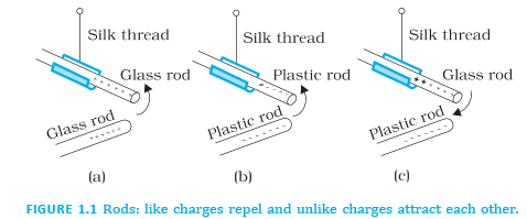
Charging by Transfer of Electrons
- Electron transfer: Rubbing transfers electrons between bodies; no new charge is created.
- Positive charge: A body becomes positively charged by losing electrons.
- Negative charge: A body becomes negatively charged by gaining electrons.
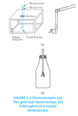
Detecting Charge: Gold-Leaf Electroscope
Conductors, Insulators and Semiconductors
Why Some Objects Charge by Rubbing
- Plastic or nylon comb: It can retain charge after rubbing dry hair because it is an insulator.
- Metal spoon: It usually does not retain charge when held because charge flows through the hand and body to the ground.
- Insulated metal: A metal rod with a wooden or plastic handle can show charging when rubbed without touching the metal.
How does rubbing a glass rod with silk charge the two objects?
Why does a held metal object usually not retain charge after rubbing?
- Like charges repel; unlike charges attract.
- Rubbing transfers electrons: losing electrons gives positive charge; gaining them gives negative charge.
- Conductors spread charge; insulators tend to keep charge localised.
Quick recap
- Electrostatics studies forces, fields and potentials due to static charges.
- There are two charge polarities: like charges repel and unlike charges attract.
- Rubbing transfers electrons; it does not create new charge.
- The gold-leaf electroscope detects charge through the divergence of its leaves.
- Conductors allow charge to move readily; insulators resist its movement.
- Semiconductors have intermediate resistance to charge movement.
Basic Properties of Electric Charge
Point charge — A charged body whose size is negligible compared with its distance from other bodies is treated as a point charge, with its charge concentrated at one point.
Additivity of charges
Additivity of charge — The total charge of a system is the algebraic sum of the charges of all its parts.
Key points
- Scalar quantity: Charge has magnitude but no direction, like mass.
- Signs matter: Unlike mass, charge may be positive or negative; include the signs when adding charges.
- System of charges: For charges , total charge is their signed sum.
- Example: in the given charge unit.
Use signed values for every charge in the system.
Conservation of charge
Conservation of charge — The total electric charge of an isolated system remains constant; charge can be transferred or redistributed, but its net amount cannot be created or destroyed.
Key points
- Rubbing: Electrons transfer from one body to another; one body gains the charge the other loses.
- Isolated system: Interactions may redistribute charge among bodies, but the system's total charge stays unchanged.
- Particle changes: Charged particles may be created or destroyed, provided total charge is conserved.
- Example: A neutron can produce a proton and an electron; their charges and sum to zero, as for the original neutron.
Quantisation of charge
Quantisation of charge — Free charge occurs in integral multiples of the elementary charge .
Here, is any integer, positive, negative or zero.
Elementary charge and SI unit
- Elementary charge: An electron has charge and a proton has charge ; (approximately ).
- Coulomb: The SI unit of charge is the coulomb, symbol ; is the charge passing a point in when current is .
- Useful scale: A charge of corresponds to about elementary charges; is therefore a large charge in many electrostatic situations.
- Smaller units: and .
This relation expresses the coulomb definition for constant current.
Why ordinary matter has quantised charge
- Matter made of protons and electrons: If a body has electrons and protons, its net charge is .
- Conclusion: Since and are integers, the body's charge is an integral multiple of and changes in steps of .
- Experimental history: Faraday's laws of electrolysis suggested charge quantisation; Millikan demonstrated it experimentally in .
| Point | Macroscopic scale | Microscopic scale |
|---|---|---|
| Typical description | Many elementary charges together appear continuous. | A few tens or hundreds of elementary charges can be counted as discrete units. |
| Role of quantisation | The step size is so small that quantisation usually has no practical effect. | The discrete steps of are important and cannot be ignored. |
Scale examples
- Electron transfer rate: If electrons move each second, the transferred charge rate is ; collecting takes about , or approximately years.
- Copper: A piece of copper contains about electrons.
- Water: A cup contains water molecules. Each molecule has protons and electrons.
- Water charge: The cup contains about of positive charge and the same magnitude of negative charge; its net charge is zero.
State the three basic properties of electric charge discussed here.
What is the net charge of a body containing electrons and protons?
Quick recap
- A point charge models a charged body whose size is negligible compared with relevant distances.
- Charges add algebraically, with positive and negative signs included.
- The total charge of an isolated system is conserved, even when charge redistributes.
- Charge is quantised: , where is an integer and .
- The SI unit is the coulomb; is approximately elementary charges.
- Quantisation is prominent at microscopic scales but usually appears continuous at macroscopic scales.
Coulomb’s Law
Coulomb’s law — The electrostatic force between two point charges acts along the line joining them, is proportional to the product of their charges, and varies inversely as the square of their separation.
Point Charges and Force Magnitude
- Point charge: A charged body can be treated as a point charge when its size is much smaller than its separation from another charge.
- Dependence: The force magnitude is proportional to and inversely proportional to .
- Direction: The force acts along the line joining the charges; like charges repel and unlike charges attract.
- Measurement: Coulomb used a torsion balance to measure forces between charged metallic spheres.
- Charge division: Contact between a charged sphere and an identical uncharged sphere divides the charge equally, enabling comparisons of charge ratios.
- Additivity and conservation: The two resulting charges, each , add to the original total charge ; charge is conserved.
- Range: Coulomb’s law has been verified from macroscopic scales down to about .
For charges and separated by distance in vacuum.
Coulomb Constant and SI Units
- Free-space permittivity: is the permittivity of free space.
- Constants: In SI units, and .
- Charge unit: Choosing this value of defines the coulomb () as the SI unit of charge.
- One-coulomb example: Two charges of separated by in vacuum exert a force of on each other.
- Practical units: The coulomb is large for many electrostatic situations; smaller units such as the millicoulomb () and microcoulomb () are used.
The Coulomb constant is written as .
Vector Form and Force Directions
- Position vectors: For charges at and , the displacement from charge to charge is ; the reverse is .
- Separation: The distance is the magnitude of either displacement: .
- Unit vectors: points from to , while points from to .
- Signed charges: The vector law uses the signed product , so one equation describes both attraction and repulsion.
The signed charge product and the unit vector from to determine the force direction.
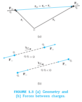
| Charge signs | Direction of force on charge 2 | Effect |
|---|---|---|
| Same sign | Along | Repulsion |
| Opposite signs | Opposite to | Attraction |
- Newton’s third law: Interchanging the charge labels gives ; the two forces are equal in magnitude and opposite in direction.
- Medium: These equations describe charges in vacuum. In matter, charged constituents affect the interaction, so the vacuum form requires modification.
State Coulomb’s law for two point charges in vacuum.
Write the vector form of the force on charge 2 due to charge 1.
Quick recap
- Treat a charged body as a point charge when its size is negligible compared with the separation.
- Coulomb force magnitude varies as .
- Charge is additive and conserved: two charges of total the original charge .
- In vacuum, .
- The signed vector law describes both attraction and repulsion.
- The forces on the two charges are equal and opposite: .
Example Based on Coulomb’s Law
Electric and Gravitational Forces
Inverse-square force — A force whose magnitude varies as the inverse square of the separation, , between two interacting objects.
The negative sign indicates attraction.
Gravity is attractive between both pairs of particles.
| Particle pair | Magnitude ratio | Force directions |
|---|---|---|
| Electron and proton | Both are attractive. | |
| Two protons | Electric force is repulsive; gravity is attractive. |
The common factor cancels, so the ratio does not depend on separation.
Forces Between Two Protons in a Nucleus
- Separation: About inside a nucleus.
- Electric force: Approximately , and repulsive.
- Gravitational force: Approximately , and attractive.
- Conclusion: At the particle scale, electric forces are enormously stronger than gravitational forces.
Acceleration of an Electron and Proton
Use , , and .
Acceleration Results
- Equal force: The electron and proton exert equal-magnitude forces on each other, but their accelerations differ because their masses differ.
- Electron: With , .
- Proton: With , .
- Implication: The Coulomb force causes very large accelerations; gravitational effects on the electron’s motion are negligible.
Effect of Changing Charge and Separation
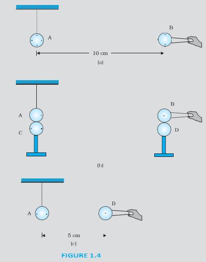
For charges and separated by distance between their centres:
Halving each charge reduces the numerator by a factor of four; halving the distance also reduces by a factor of four. The force is unchanged.
Why is the electric force between an electron and proton so much stronger than their gravitational force?
The electron and proton experience equal-magnitude forces. Why are their accelerations different?
Quick recap
- Electric and gravitational forces both follow an inverse-square law.
- Electric forces greatly exceed gravitational forces between elementary particles.
- Two protons repel electrically but attract gravitationally.
- At a separation of , the electron and proton experience a force of .
- Equal and opposite interaction forces can produce different accelerations because the masses differ.
- Halving both charges and the separation leaves the Coulomb force unchanged.
Forces Between Multiple Charges
Principle of Superposition
Principle of superposition — The net electrostatic force on a charge due to several other charges is the vector sum of the forces exerted by each charge separately.
Key points
- One charge at a time: Calculate each force using Coulomb’s law as if the other charges were absent.
- Unaffected forces: The presence of additional charges does not alter any individual pairwise force.
- Vector addition: Add all individual forces using vector addition, such as the parallelogram law.
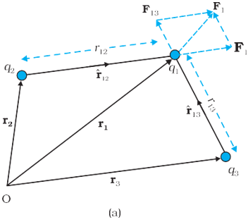
Calculating the Net Force
Forces on a charge
- Pairwise force: For charges and , separated by distance , Coulomb’s law gives the force on due to .
- Direction: The force acts along the line joining the charges; its direction depends on whether the charges attract or repel.
- Net force: The total force on is the sum of all pairwise force vectors.
Here, points from toward .
For charges, add the forces from through .
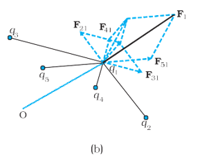
Using the principle
- Procedure: Find each force’s magnitude and direction, then add the vectors to obtain the resultant.
- Symmetry: In arrangements such as equal charges at the vertices of an equilateral triangle, use the force directions and symmetry when finding the resultant.
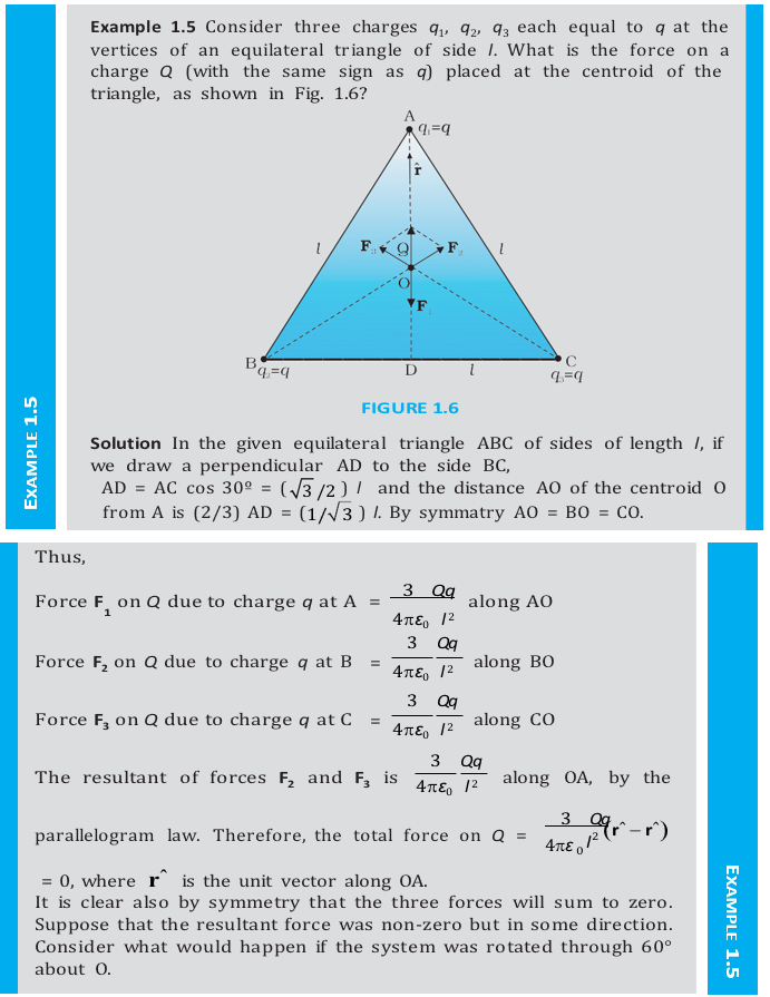
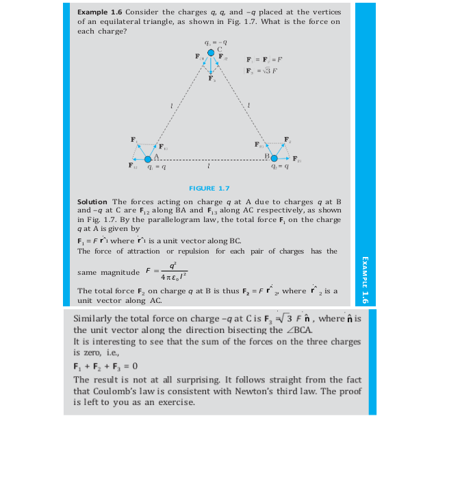
Do not add force magnitudes alone when the forces point in different directions; the net force is a vector sum.
State the principle of superposition for electrostatic forces.
How do you find the net force on in a system of charges?
Quick recap
- The net electrostatic force is the vector sum of individual Coulomb forces.
- Each pairwise force is unchanged by the presence of other charges.
- Calculate forces one pair at a time, keeping their directions.
- For charges, the force on is .
- Use symmetry and vector addition to determine the resultant force.
Electric Field
Electric Field of a Point Charge
Source Charge and Test Charge
- Source charge : Produces the electric field and should remain at its original position.
- Test charge : A charge used to determine the field by measuring the force on it.
- Test-charge limit: Choose negligibly small so it does not disturb the source; the ratio remains finite.
- SI unit: From , electric field is measured in newtons per coulomb ().
Direction and Symmetry
- Positive source: The electric field points radially outward.
- Negative source: The electric field points radially inward.
- Spherical symmetry: For a point charge, field magnitude depends only on distance ; it is equal everywhere on a sphere centred on the charge.
- Independence from test charge: Since force is proportional to , the ratio and hence the source field do not depend on the test charge.
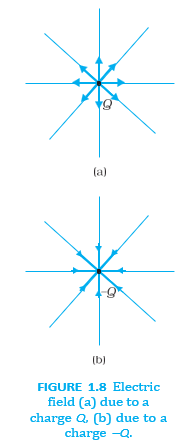
Keeping the Source Undisturbed
- Ideal approach: Use a negligibly small test charge so its effect on the source is negligible.
- Practical approach: The source charge can be held in place by other forces; charges in a charged sheet, for example, are held by forces from the sheet’s constituents.
Electric Field Due to a System of Charges
Superposition Principle
- Individual contribution: Each charge produces its own electric field at the field point, directed along the line from that charge to the point.
- Net field: Add the individual fields as vectors; the original source charges are not disturbed.
- Distance and direction: For charge , use its distance from point and the unit vector pointing from to .
Physical Significance of Electric Field
What the Field Represents
- Electrostatics: The field is a convenient way to describe the electrical environment created by a charge system; the measurable effect is the force on a charge.
- Field at a point: It tells the force that a unit positive test charge would experience there, without disturbing the source system.
- Vector field: Electric field is defined at every point in space and can vary from point to point; it is a vector because force is a vector.
- System property: The field characterises the source charges and is independent of the test charge used to measure it.
Why Fields Matter for Changing Charges
- An accelerated charge produces changing electromagnetic fields.
- The influence propagates outward as electromagnetic waves at the speed of light, .
- The waves reach another charge after a time delay and exert a force on it.
Fields as Physical Entities
- Independent dynamics: Electromagnetic fields evolve according to laws of their own; they are not merely mathematical descriptions of forces.
- Energy transport: Propagating electromagnetic fields can carry energy, even after the source has stopped changing.
- Origin of the concept: The concept of field was introduced by Faraday.
Do not treat electric field as depending on the test charge: the force depends on , but the source field does not.
Define electric field and state its SI unit.
State the superposition principle for electric fields.
Quick recap
- A point charge produces a field .
- The force on a charge in a field is ; the SI field unit is .
- The field is defined using a negligibly small test charge and is independent of that test charge.
- Fields point outward from positive charges and inward toward negative charges; a point charge has spherical symmetry.
- Fields from multiple charges add vectorially by superposition.
- Changing electromagnetic fields propagate at speed , can cause delayed forces, and transport energy.
Example Based on Electric Field
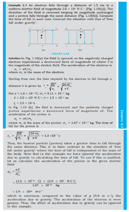
Charged Particles Between Oppositely Charged Plates
Electric Field of a Point Charge
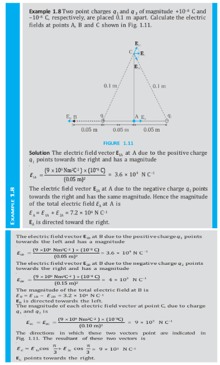
Quick recap
- The lecture illustrates an electron and a proton accelerating between oppositely charged plates.
- The plate illustration includes reversed electric-field cases.
- A second illustration shows a point-charge electric field at points A, B, and C.
- For a point charge, the electric field is radial, with magnitude E = |Q|/(4πε₀r²); it points outward for positive charge and inward for negative charge.
Electric Field Lines
Representing the Electric Field
Field-line representation
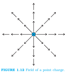
- Vector field: The electric field has direction and magnitude; arrows can represent it at different points.
- Arrow length: Draw each arrow with length proportional to the electric-field strength at that point.
- Force meaning: An electric-field vector gives the force on a unit positive charge placed at its tail.
- Point charge: For a positive point charge, field arrows point radially outward and get shorter farther from the charge as the field weakens.
- Field line: A curve drawn so that its tangent at each point gives the direction of the net electric field there.
- Arrow and space curve: An arrow shows which tangent direction is the field direction; field lines are three-dimensional curves, even when drawn in a plane.
Field-Line Density and Strength
- Direction: The tangent to a field line gives the electric-field direction at that point.
- Relative strength: Field strength is represented by the relative density of lines—the closer the lines, the stronger the field.
- Crowding: Lines are crowded near a point charge, where the field is stronger, and spread farther apart as the field weakens.
- Relative, not absolute: The number of lines drawn is arbitrary; compare their density in different regions rather than counting them.
- Density measure: In three dimensions, compare the number of lines crossing a unit area perpendicular to the field.
The density is measured as lines crossing unit area perpendicular to the field; it indicates relative field strength.
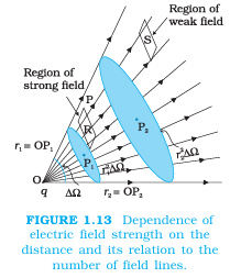
Solid Angle and Inverse-Square Dependence
Solid angle — A three-dimensional measure of a cone; for a small perpendicular area on a sphere of radius , it is the area divided by .
A small transverse length at distance subtends this angle.
A small area , perpendicular to the radius at distance , subtends this solid angle.
Why the field of a point charge varies as inverse square
- For a fixed solid angle, the same number of radial field lines crosses the corresponding area at every distance.
- The area subtending that solid angle grows as .
- Thus, the number of lines per unit area—and hence the field strength—decreases as .
The field magnitude varies inversely with the square of the distance from the charge.
Field Lines Around Charge Configurations
Origin and meaning
- Faraday: Introduced the field-line picture as a visual, non-mathematical way to represent electric fields; he called them “lines of force.”
- Preferred term: “Field lines” is more appropriate because “lines of force” can be misleading, especially for magnetic fields.
- Positive charge: Field lines point radially outward from a single positive charge.
- Negative charge: Field lines point radially inward toward a single negative charge.
- Charge pairs: The pattern for two positive charges depicts their mutual repulsion; the dipole pattern for and depicts attraction.
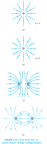
General Properties of Electric Field Lines
- Starting and ending points: Field lines start on positive charges and end on negative charges; for an isolated charge, they may begin or end at infinity.
- Continuity: In a charge-free region, field lines are continuous curves with no breaks.
- No crossing: Two field lines cannot intersect, because the field at an intersection would have two directions.
- No closed loops: Electrostatic field lines do not form closed loops, because the electrostatic field is conservative.
How do field lines show the direction and relative strength of an electric field?
Why can two electric field lines never cross?
Quick recap
- Field arrows are drawn with lengths proportional to electric-field strength; the field-line tangent and arrow show its direction.
- Closer field lines mean a stronger field; their absolute number is arbitrary.
- For a point charge, field strength varies as because area per fixed solid angle grows as .
- Lines point away from positive charges and toward negative charges.
- Field lines are continuous in charge-free regions, never cross, and do not form closed loops.
Electric Flux
Meaning of Electric Flux
- Electric flux: A measure of how much electric field passes through a surface; it is analogous to the flow of a liquid, but no physical substance flows.
- Field strength: Flux through a surface depends on the electric field and the surface’s orientation.
Area Vector
- Area vector: A planar area is represented by a vector whose magnitude is the area and whose direction is normal to the plane.
- Curved surface: Divide it into small, approximately planar area elements, each with its own area vector.
- Closed surface: By convention, each area vector points along the outward normal.
Flux Through a Surface Element
- Electric flux: Through a small area element, ");
- Angle: In the flux expression, is the angle between the electric field and the area vector; flux is greatest when they are parallel and zero when they are perpendicular.
- SI unit: Electric flux is measured in N·m²/C.
Total Flux Through a Surface
Use this form for the exact total flux through a surface.
Quick recap
- Electric flux measures the electric field passing through a surface; it is not a physical flow.
- The area vector has magnitude equal to the area and points normal to the surface.
- For a closed surface, each area vector points outward.
- Flux through an element is .
- The SI unit of electric flux is .
- Total flux is the sum over small elements, or exactly .
Electric Dipole
Electric dipole and dipole moment
Electric dipole — A pair of equal and opposite point charges, and , separated by distance .
- Dipole axis: The line joining the two charges; the dipole direction is from to .
- Centre: The midpoint between the charges. The dipole has zero net charge, but its electric field is generally non-zero.
- Far field: At distances much greater than the separation, the two charge fields nearly cancel; the dipole field decreases as , faster than a single-charge field ().
Electric dipole moment — A vector equal to the charge magnitude multiplied by the separation, directed from the negative charge to the positive charge.
Its magnitude is ; its direction is from to .
Electric field of a dipole
- Method: Find the fields due to and using Coulomb’s law, then add them as vectors using superposition.
- Special positions: The axial point lies on the dipole axis; the equatorial point lies in the plane perpendicular to that axis through the dipole centre.
Field on the dipole axis
- Point location: For a point at distance from the centre on the side, its distances from and are and .
- Direction: The net field points along the dipole moment direction, from towards .
For a point on the side of the dipole:
When , express the result using dipole moment :
Field on the equatorial plane
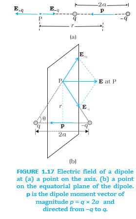
- Geometry: Each charge is at distance from a point on the equatorial plane, so the two field magnitudes are equal.
- Components: Components perpendicular to the dipole axis cancel; components along the axis add.
- Direction: The net field points opposite to the dipole moment.
The field is opposite to :
When :
- Axial far field: , along .
- Equatorial far field: , opposite to .
- Distance dependence: A dipole’s far field varies as and depends on direction as well as distance.
Point dipole — An ideal dipole whose separation tends to zero and charge magnitude tends to infinity while its dipole moment remains finite.
For a point dipole, the axial and equatorial field expressions above are exact at any non-zero distance.
Physical significance of dipoles
| Molecule type | Charge centres | Examples and dipole behaviour |
|---|---|---|
| Non-polar | Positive and negative charge centres coincide. | CO₂ and CH₄ have zero dipole moment without an applied field; an electric field can induce a dipole moment. |
| Polar | Positive and negative charge centres do not coincide. | H₂O has a permanent electric dipole moment, even without an applied field. |
The charge-weighted position is analogous to the centre of mass:
Define the electric dipole moment and state its direction.
How do the far-field directions and magnitudes compare on the axis and equatorial plane?
What distinguishes polar from non-polar molecules?
Quick recap
- An electric dipole consists of equal and opposite charges separated by a finite distance.
- Dipole moment is , directed from negative to positive charge.
- On the axis, the far field is along and has magnitude .
- On the equatorial plane, the far field is opposite to and has magnitude .
- A dipole’s far field falls as ; point-dipole fields are exact in the ideal limit.
- Polar molecules have permanent dipole moments; non-polar molecules can acquire induced moments in an electric field.
Dipole in a Uniform External Field
Electric Dipole in a Uniform External Field
Permanent dipole — A dipole with dipole moment that exists independently of an external electric field.
Torque in a Uniform Field
- Forces: The charges and experience equal and opposite forces, and ; hence the net force on the dipole is zero.
- Torque: Since the forces act at separated points, they form a couple. Its torque tends to rotate the dipole to align with .
- Direction: The torque is perpendicular to the plane containing the dipole axis and the field, in the direction given by the right-hand rule.
For charges separated by , with angle between and , the torque magnitude is .
- Magnitude: ; torque is zero when the dipole is parallel or antiparallel to the field.
- Stable alignment: The torque tends to align the dipole moment with the field.
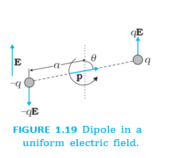
Dipole in a Non-Uniform Electric Field
- Net force: In a non-uniform field, the forces on the two charges are unequal, so the dipole can experience a net force.
- Parallel orientation: If is parallel to , the net force is toward the region of increasing field strength.
- Antiparallel orientation: If is antiparallel to , the net force is toward the region of decreasing field strength.
- General orientation: The force depends on the dipole’s orientation relative to the field; a torque may also act.
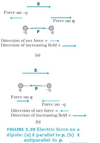
Why a Charged Comb Attracts Paper
- Polarisation: A charged comb induces a net dipole moment in an initially uncharged piece of paper, oriented along the comb’s field.
- Attraction: The comb’s field is non-uniform, so the induced dipole experiences a net force toward the comb.
Continuous Charge Distribution
Continuous charge distribution — A macroscopic model in which charge is treated as smoothly spread over a line, surface, or volume rather than as separate microscopic charges.
- Why use it: For many physical systems, specifying every microscopic charge is impractical; instead, use small macroscopic elements containing many charges.
- Averaging: Charge density smooths over microscopic discreteness and quantisation, in the same way macroscopic mass density treats matter as continuous.
- Densities: Linear, surface, and volume charge densities describe charge per unit length, area, and volume, respectively.
| Density | Definition | SI unit |
|---|---|---|
| Linear, | ||
| Surface, | ||
| Volume, |
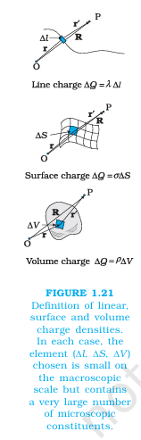
Electric Field of a Continuous Distribution
- Elemental charge: A small volume element at position contains charge .
- Field contribution: At a point with position vector , this element produces a field along the unit vector from the element toward .
- Superposition: Add the field contributions of all volume elements; in the continuous limit, the sum becomes an integral.
Here, is the distance from the charge element to , and points from the element toward .
Sum over all volume elements; as their sizes tend to zero, use the corresponding integral.
- Use for dipole torque; a uniform field gives zero net force but can give non-zero torque.
- A non-uniform field can exert a net force on a dipole, including an induced dipole.
- Continuous-distribution fields follow Coulomb’s law and the superposition principle, with a sum replaced by an integral in the limit.
Why does a dipole experience torque in a uniform electric field even though its net force is zero?
Why is an uncharged piece of paper attracted to a charged comb?
Define linear, surface, and volume charge density.
Quick recap
- A permanent dipole in a uniform field has zero net force but generally experiences torque.
- Dipole torque is , with magnitude .
- In a non-uniform field, a dipole can experience a net force depending on its orientation.
- A charged comb attracts uncharged paper by inducing a dipole in the paper within a non-uniform field.
- Linear, surface, and volume charge densities are charge per unit length, area, and volume.
- The field of a continuous charge distribution is found by summing the fields of its elements, or integrating in the continuous limit.
Gauss’s Law
Flux Through a Sphere Enclosing a Point Charge
- Setup: A point charge is at the centre of a sphere of radius . The electric field is radial and has the same magnitude everywhere on the sphere.
- Area direction: Each area vector points radially outward, parallel to the field for a positive charge.
- Flux element: The flux through each small area is , since the field and area vector are parallel.
- Total flux: The field magnitude is constant over the sphere, so the total flux is the field magnitude multiplied by the sphere’s area.
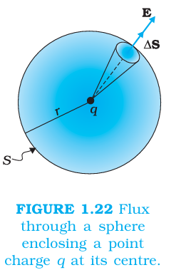
Using Coulomb’s law and the sphere’s area, the radius dependence cancels.
Statement and Meaning of Gauss’s Law
Gauss’s law — The total electric flux through any closed surface equals the net charge enclosed divided by the permittivity of free space.
Here is the algebraic sum of charges enclosed by the surface.
- Zero enclosed net charge: The net flux through a closed surface is zero when its total enclosed charge is zero; enclosed positive and negative charges may still be present if they cancel.
- Charge outside: Outside charges contribute to the electric field on the surface and therefore to the flux calculation, but not to .
- Generality: Gauss’s law holds for every closed surface, regardless of its shape or size; enclosed charges may lie anywhere inside it.
Zero Flux in a Uniform Electric Field
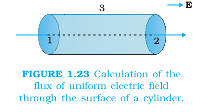
- Curved side: Its outward normal is perpendicular to the field, so the flux through the curved surface is zero.
- End caps: The field enters one cap and leaves the other. For equal cap areas , their fluxes are and .
- Net result: The total flux is zero, consistent with zero net charge enclosed.
Gaussian Surfaces and Applications
Gaussian surface — An imaginary closed surface chosen to apply Gauss’s law.
- Choice of surface: Any closed shape can be used; a surface chosen to match the system’s symmetry often makes the electric-field calculation easier.
- Discrete charges: Do not let a Gaussian surface pass through a discrete charge, where the field is not defined. It may pass through a continuous charge distribution.
- Inverse-square basis: Gauss’s law depends on the inverse-square distance dependence in Coulomb’s law; a violation would indicate departure from this law.
What does the charge on the right-hand side of Gauss’s law represent?
Why is the net flux through a closed cylinder in a uniform parallel field zero?
Quick recap
- Gauss’s law relates closed-surface flux to the net enclosed charge: .
- A sphere around a point charge has total flux , independent of its radius.
- The field in the flux integral is due to all charges; only enclosed charges count on the law’s right-hand side.
- Zero net flux means zero net enclosed charge, not necessarily an absence of charges.
- Choose a Gaussian surface that matches symmetry, and do not pass it through a discrete charge.
Applications of Gauss’s Law
Using Gauss’s Law
Gauss’s law — The net electric flux through a closed surface equals the enclosed charge divided by .
When Gauss’s Law Is Useful
- Use: It is especially effective for symmetric charge distributions, where symmetry simplifies the electric field.
- Gaussian surface: Choose a closed surface that matches the charge distribution’s symmetry.
- General distributions: The integration needed to find the field is usually difficult except in special cases.
Field Due to an Infinitely Long Uniformly Charged Wire
Linear charge density — Linear charge density is the charge per unit length of a wire.
Symmetry and Gaussian Surface
- Direction: The field is radial, outward for and inward for .
- Magnitude: It is the same at every point the same radial distance from the wire, and does not vary along the wire.
- Gaussian surface: Use a coaxial cylinder of radius and length ; the field is perpendicular to its curved surface.
- Flux and enclosed charge: The flat ends have zero flux; the curved area is , and the enclosed charge is .
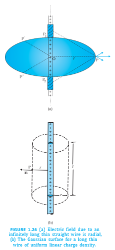
Here is radial and lies in the plane perpendicular to the wire. The sign of gives the field direction.
The field is caused by the entire wire, although the Gaussian cylinder encloses only . The infinite-wire assumption matters; for a long finite wire, the result is approximate near its middle, where end effects are negligible.
Field Due to a Uniformly Charged Infinite Plane Sheet
Surface charge density — Surface charge density is the charge per unit area of a sheet.
Symmetry and Gaussian Surface
- Direction: The field is perpendicular to the sheet and has equal magnitude on both sides.
- Distance: The field is independent of distance from an infinite sheet.
- Gaussian surface: Use a pillbox of face area crossing the sheet.
- Flux and enclosed charge: Only the two flat faces contribute, giving total flux ; the enclosed charge is .
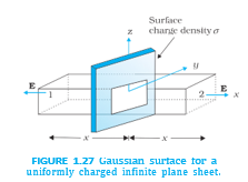
The unit normal points away from the sheet. The field points away for and toward the sheet for .
Finite-Sheet Approximation
- Large finite sheet: The infinite-sheet result is approximately valid in the middle region, away from the edges.
Field Due to a Uniformly Charged Thin Spherical Shell
Spherical Symmetry
- Field pattern: The field is radial, and its magnitude depends only on distance from the shell’s centre.
- Total charge: For shell radius and uniform surface charge density , the shell’s charge is .
Field Outside the Shell
- Gaussian surface: A concentric sphere of radius has constant radial field over its surface.
- Flux: The total flux is ; the enclosed charge is the full shell charge .
- Result: Outside, the shell’s field is the same as that of a point charge placed at its centre.
Field Inside the Shell
- Gaussian surface: For a concentric sphere with , the enclosed charge is zero.
- Result: Gauss’s law gives , so the field is zero everywhere inside the shell.
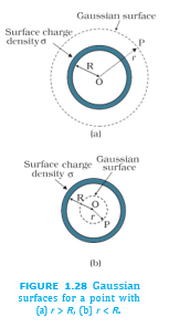
Outside the shell, the field points outward for and inward for ; inside, it is zero.
Signed Vector Components
- Signed scalar: In , a positive points along ; a negative points opposite to it.
- Modulus: The magnitude is non-negative.
Significance of the Zero-Field Result
- Consequence: The zero field inside a uniformly charged thin shell follows from Gauss’s law, which follows from Coulomb’s law.
- Experimental significance: Verifying this result experimentally confirms the inverse-square dependence in Coulomb’s law.
Why is a cylindrical Gaussian surface suitable for an infinitely long charged wire?
State the field due to an infinite uniformly charged plane sheet.
What is the field inside a uniformly charged thin spherical shell, and what does verifying this result confirm?
Quick recap
- Gauss’s law is most useful for symmetric charge distributions.
- An infinite line charge produces a radial field .
- An infinite plane sheet produces a normal field , independent of distance.
- Outside a uniformly charged spherical shell, the field is equivalent to that of a point charge at its centre.
- Inside a uniformly charged thin spherical shell, the electric field is zero.
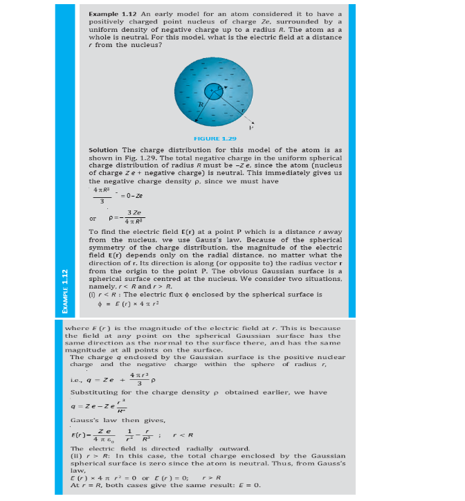
- The spherical atom diagram shows a positive nucleus, distributed negative charge, and a point at distance .
Summary
Electric Charge and Its Properties
Three basic properties of charge
- Quantisation: A body's charge is an integral multiple of the elementary charge: , where . A proton has charge and an electron .
- Macroscopic charges: When is very large, quantisation is usually negligible in practice. Charge quantisation is a basic law of nature; there is no analogous law for mass.
- Additivity: Total charge is the algebraic sum of individual charges, including their signs. Charge is a scalar.
- Conservation: The total charge of an isolated system remains constant. Charging by friction transfers charge; it does not create or destroy it.
Charge invariance and conservation
- Invariance: Charge is unchanged by rotation and by changing to a frame moving relative to the original frame.
- Distinct ideas: Conservation means constancy with time in an isolated system; it is not the same as being a scalar. A scalar need not be conserved, and a vector quantity can be conserved.
Coulomb’s Law and Superposition
Force on due to ; points from to .
SI units and constants
- Charge unit: The SI unit is the coulomb; .
- Permittivity: .
- Coulomb constant: . In SI, the ampere is defined via its magnetic effect and the coulomb follows from , fixing ; the coulomb is a large unit for electric effects.
| Point | Electric force | Gravitational force |
|---|---|---|
| Magnitude between a proton and an electron | About times the gravitational force | Much weaker at the particle scale |
| Sign and large-scale effect | Can attract or repel, so positive and negative contributions can cancel | Always attractive; therefore can dominate on large scales despite its weakness |
| Distance dependence | Inverse-square law | Inverse-square law |
For an electron and a proton separated by the same distance.
Superposition principle — Each pairwise force is unaffected by other charges, and the net force is the vector sum of all pairwise forces; no additional forces arise only when three or more charges are present.
Add the forces due to all other charges as vectors.
Electric Field and Field Lines
At distance from a point charge ; the field points outward for and inward for .
Field superposition and where the field is defined
- Superposition: The net electric field is the vector sum of the fields due to all charges.
- Discrete charges: The field of a discrete charge configuration is undefined at the locations of its charges.
- Continuous distributions: For a continuous volume charge distribution, the field is defined at every point within the distribution.
- Surface charge: The electric field is discontinuous across a surface charge distribution.
Electric field line — A curve whose tangent at each point gives the direction of the electric field there.
Field-line properties
- Strength: Closer lines indicate a stronger field; widely spaced lines indicate a weaker field. A uniform field has parallel, equally spaced straight lines.
- Continuity: Electrostatic field lines are continuous curves with no breaks.
- No crossing: Two field lines cannot cross because the field has a unique direction at each point.
- Start and end: Lines begin on positive charges and end on negative charges; electrostatic field lines do not form closed loops.
Electric Dipole
Dipole moment
- Magnitude and direction: ; the vector points along the dipole axis from to .
- Distant dipole field: For a dipole, the field decreases as , faster than the field of a point charge.
At distance from the centre, for ; the field is opposite to .
For a point on the axis outside the charges (), these are field magnitudes. The field points along on either exterior side of the dipole.
Dipole in a uniform electric field
- Torque: A dipole experiences torque .
- Net force: A dipole in a uniform electric field experiences no net force.
Electric Flux and Gauss’s Law
The dot product accounts for the angle between the field and the area normal. For a closed surface, the area normal is outward by convention.
Gauss’s law — The total electric flux through any closed surface equals the total charge enclosed divided by .
Especially useful for finding fields when the charge distribution has simple symmetry.
| Distribution | Electric field | Conditions and direction |
|---|---|---|
| Infinite straight wire with uniform linear charge density | is the perpendicular distance from the wire; direction is radial in the plane normal to it. | |
| Infinite plane sheet with uniform surface charge density | Normal to the plane, outward on either side for a positive sheet. | |
| Thin spherical shell of radius and total charge | for ; for | Outside, the field is as if all charge were concentrated at the centre; inside, it is zero. |
Spherical charge distributions
- Shell charge: For uniform surface charge density , the shell charge is .
- Uniform solid sphere: Its external field is the same as that of a point charge equal to its total charge, placed at the centre.
| Quantity | Symbol | Dimensions | SI unit |
|---|---|---|---|
| Vector area element | |||
| Electric field | |||
| Electric flux | |||
| Electric dipole moment | |||
| Linear charge density | |||
| Surface charge density | |||
| Volume charge density |
Further conceptual points
- Nuclear structure: The short-range strong force, effective over roughly , holds protons together in the nucleus. Quantum mechanics prevents electrons from residing inside the nucleus.
- Zero total charge: A configuration with zero total charge need not have zero electric field. At large distances, its field can fall faster than ; a dipole is the simplest example.
- Gravity and electric cancellation: Both forces follow an inverse-square law, but electric forces can cancel because they have two signs, whereas gravity is always attractive.
State Coulomb’s law and give the SI value of its constant.
What does Gauss’s law state?
How does an electric dipole behave in a uniform electric field?
Quick recap
- Charge is quantised, additive and conserved; like charges repel and unlike charges attract.
- Coulomb’s law gives the force between point charges; superposition adds pairwise forces as vectors.
- Electric field is force per unit positive test charge; field-line direction and spacing show field direction and relative strength.
- A dipole moment points from negative to positive charge; its distant field varies as .
- Electric flux is ; Gauss’s law connects closed-surface flux to enclosed charge.
- Gauss’s law gives simple field results for an infinite wire, infinite sheet and spherical shell.
- For a continuous volume charge distribution, the field is defined at every point within the distribution.
Physics — ALL CHAPTERS
1
Electric Charges And Fields
2
Electrostatic Potential And Capacitance
3
Current Electricity
4
Moving Charges And Magnetism
5
Magnetism And Matter
6
Electromagnetic Induction
7
Alternating Current
8
Electromagnetic Waves
1
Ray Optics And Optical Instruments
2
Wave Optics
3
Dual Nature Of Radiation And Matter
4
Atoms
5
Nuclei
6
Semiconductor Electronics: Materials, Devices And Simple Circuits