Class 9 . Mathematics . Ganita Manjari . Introduction to Linear Polynomials
Chapter 2: Introduction to Linear Polynomials
Ch 2
Mathematics
Class 9
Introduction
Algebraic Expressions: Terms, Variables and Coefficients
Algebraic expression — A mathematical expression made from numbers, variables and operations such as addition and multiplication.
Parts of an expression
- Term: A part of an expression separated by or ; the terms in are , and .
- Variable: A letter representing a number, such as or ; it is also called a letter-number.
- Coefficient: The numerical factor multiplying a variable; the coefficients of and in are and .
- Constant: A term with no variable; the constant in is .
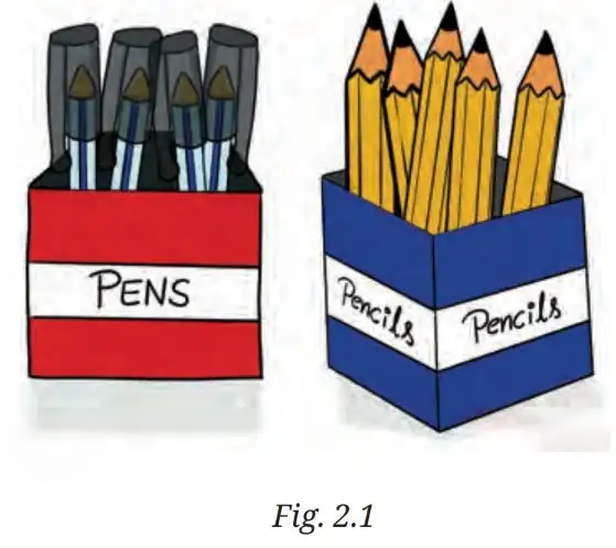
For red boxes with pens each, blue boxes with pencils each, and extra pens:
Raju buys red boxes containing pens each and blue boxes containing pencils each. He also receives extra pens. Write the total quantity.
- Multiply the red-box count by the pens in each box.
- Multiply the blue-box count by the pencils in each box.
- Add the free pens to the two quantities.
Identify the parts of an expression
- Separate the terms at each plus or minus sign.
- Identify the letters that represent variables.
- Read the numerical multiplier of each variable term as its coefficient.
- Identify any term without a variable as a constant.
Expressions from situations
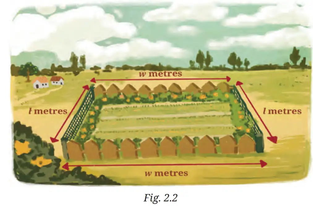
- Garden fencing: A rectangular garden has length metres and width metres. Length fencing costs Rs. 100 per metre and width fencing costs Rs. 80 per metre.
- Wire fence cost: Fencing both lengths costs rupees.
- Wooden fence cost: Fencing both widths costs rupees.
- Seed cost: The area is , so seeds at Rs. 50 per square metre cost rupees.
- Total cost: ; its terms are , and , and its variables are and .
Polynomials in One Variable and Their Degree
Polynomial in one variable — An algebraic expression involving one variable and its non-negative whole-number powers; it is also called a univariate polynomial, or simply a polynomial when the context is clear.
Polynomial examples and terminology
- Univariate: This word means “having one variable”; examples include , , and .
- Coefficients: In , the coefficients of , and are , and ; the constant term is .
- Degree: The highest power of the variable in a polynomial is its degree.
The degree is the highest power of the variable with a non-zero coefficient. Degree polynomials are cubic, degree are quadratic, degree are linear, and non-zero degree polynomials are constant. For example, , so the non-zero constant polynomial has degree .
The leading coefficient satisfies ; the exponents are non-negative whole numbers.
| Polynomial | Degree | Type |
|---|---|---|
| Cubic | ||
| Quadratic | ||
| Linear | ||
| Constant |
| Point | One variable | Multiple variables |
|---|---|---|
| Variables present | One, such as | Two or more, such as and |
| Example |
Rectangle area as a polynomial
- Perimeter: A wire of length cm forms a rectangle, so . If its length is cm, its width is cm.
- Area: The area expression is , a polynomial in one variable.
Find a polynomial's degree and type
- Check that the expression has one variable and only non-negative whole-number powers.
- Write the terms in descending powers if needed.
- Find the highest power with a non-zero coefficient.
- Name it using its degree: cubic, quadratic, linear or constant.
Determine the degree and type of .
- The expression contains only the variable ; its powers are non-negative whole numbers.
- The highest power of is .
- A degree- polynomial is cubic.
Do not use the number of terms to find degree. Use the highest power: has degree because its highest power is .
For , state the variable, terms, coefficients of the variable terms, constant and degree.
A rectangle has perimeter cm and length cm. Write its area as a polynomial in and state its degree.
Quick recap
- An algebraic expression has terms, variables, coefficients and possibly a constant.
- The garden cost expression is and involves two variables.
- A polynomial in one variable is also called a univariate polynomial; “univariate” means having one variable.
- The degree of a polynomial is its highest variable power with a non-zero coefficient.
- Degree , and polynomials are linear, quadratic and cubic, respectively.
- A non-zero constant polynomial such as has degree because .
Linear Polynomials
Linear Patterns
Linear pattern — A pattern is linear when its values change by a constant amount for equal increases in the input.
For a linear polynomial, the difference between successive values at inputs increasing by is constant. For other equal input steps, the change is also constant.
For side length , the perimeter is a linear polynomial.
What are the perimeters of squares with sides , , , and cm?
- Find the perimeters for side lengths increasing by cm.
- Substitute the given side lengths.
- Each cm increase in side length raises the perimeter by cm.
| Matches played | 1 | 2 | 3 | 4 | 5 | |
|---|---|---|---|---|---|---|
| Amount paid (Rs.) | 250 | 300 | 350 | 400 | 450 |
The joining fee is Rs. 200, plus Rs. 50 for each match played.
Find matches from the total cost
- Subtract the fixed joining fee from the total paid.
- Divide the remainder by the cost per match.
A player paid Rs. 750. How many matches did the player play?
- Substitute the total cost of Rs. 750.
- Subtract Rs. 200 and divide by Rs. 50.
Linear Equations
Linear equation — A linear equation is formed by equating a linear polynomial in one variable to a constant.
Translate a word problem into a linear equation
- Choose a variable for the unknown quantity.
- Express the other quantities using that variable.
- Use the stated relationship to form and solve the equation.
The sum of two numbers is . One number is more than the other. Find the numbers.
- Let the smaller number be ; the larger is more.
- Set their sum equal to and simplify.
- Solve for the smaller number.
- Add to get the larger number.
Polynomials as Input–Output Processes
Function — A function assigns an output to each input; a polynomial can define a function by substituting the input value into its expression.
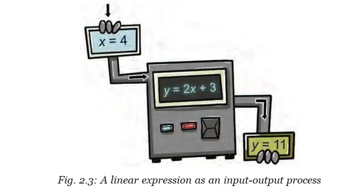
The expression gives one output for each value of .
| Point | Linear | Quadratic |
|---|---|---|
| Example | ||
| Degree | 1 | 2 |
Evaluate at and . Also find at cm.
- Evaluate the linear polynomial at .
- Evaluate it at .
- The rectangle-area expression is evaluated by the same substitution process.
A square has side cm. Find its perimeter.
A club charges Rs. 200 to join and Rs. 50 per match. Find the cost for matches.
Evaluate when .
Quick recap
- A linear pattern has a constant change for equal steps in the input.
- A square with side has perimeter .
- The chess club cost for matches is .
- Equating a linear polynomial to a constant forms a linear equation.
- A polynomial function maps each input to an output by substitution.
- is linear, while is quadratic.
Exploring linear patterns
Growing Square-Tile Pattern
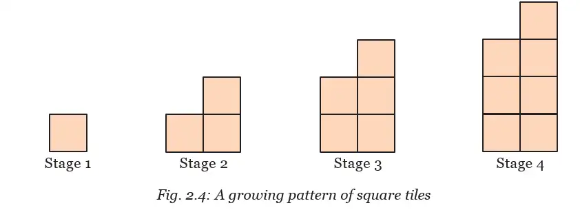
| Stage | 1 | 2 | 3 | 4 | 5 | 6 | 7 |
|---|---|---|---|---|---|---|---|
| Number of tiles | 1 | 3 | 5 | 7 | 9 | 11 | 13 |
Pattern observations
- Sequence: The tile counts are .
- Increase: Each new stage adds tiles, so consecutive terms have a constant difference of .
- Rule: The count at each stage is one less than twice the stage number.
Linear polynomial — A polynomial of degree is called a linear polynomial.
The number of tiles at Stage is , a degree- polynomial. Its constant increase of gives a linear relationship between stage number and tile count.
Use this rule to find the tile count at any stage.
Use a linear pattern rule
- Substitute the stage or term number into the rule.
- To find the stage for a target count, equate the rule to that count.
- Solve for the stage number and check that it is a valid stage.
How many square tiles are in Stage 15?
- Substitute Stage into the tile rule.
Pocket-Money Pattern
| Day number | 0 | 1 | 2 | 3 | 4 |
|---|---|---|---|---|---|
| Amount left | ₹100 | ₹95 | ₹90 | ₹85 | ₹80 |
Pocket-money rule
- Starting amount: Bela has ₹100 and spends ₹5 each day.
- Daily change: The amount remaining decreases by ₹5 per day.
- Rule: After days, subtract the total spending from the starting amount.
Use to calculate the amount remaining after days.
Find the remaining amount or number of days
- Use the daily spending rule for the given day number.
- For a target amount, set the rule equal to that amount and solve for .
After how many days will Bela have ₹40 left?
- Set the amount remaining equal to ₹40.
- Solve for the number of days.
Auto-Rickshaw Fare Pattern
Fare rule
- Initial fare: The fare is ₹25 for the first 2 km.
- Increase: After 2 km, the fare rises by ₹15 for each additional kilometre.
- Example: For 10 km, add the charge for the 8 km travelled beyond the initial 2 km.
For distances of at least km, the fare is a linear function of distance.
Calculate a fare or find the distance
- For a given distance, substitute it into the fare rule.
- For a given fare, set the expression equal to the fare and solve for .
What is the fare for a travel of 10 km?
- Use the fare rule for a journey of 10 km.
Linear pattern — A linear pattern is a sequence in which the difference between consecutive terms is constant; its term can be expressed as a linear expression in the term number.
For the tile pattern, find the number of tiles at Stage 26 and the stages containing 21 and 47 tiles.
How much money remains after 15 days, and after how many days will Bela have spent the entire ₹100?
For what distance will the auto-rickshaw fare be ₹130?
For the auto-rickshaw fare, add ₹15 only for kilometres beyond the first 2 km. Use , not ₹25 plus ₹15 times the whole distance.
Quick recap
- A linear pattern has a constant difference between consecutive terms.
- The tile sequence has common difference and rule .
- The rule is a degree- polynomial, so it is a linear polynomial.
- Bela's remaining money after days is given by ; she has ₹40 after 12 days.
- For , the auto-rickshaw fare is .
Linear growth and linear decay
Linear Expressions as Models
How linear expressions model change
- Use: Linear expressions can model real situations in which a quantity grows or declines.
- Pattern: A linear model changes by a constant amount over equal intervals of the input.
Linear Growth
Linear growth — A quantity shows linear growth when it increases by a constant amount over equal intervals.
Key points
- Pattern: Equal increases in the input produce equal increases in the output.
- Rate: The constant increase per interval is the growth rate.
- Journey cost: The starting charge is Rs. 100, and the cost rises by Rs. 60 per kilometre.
For each increase of km in distance, the journey cost increases by Rs. 60.
Here, is distance in kilometres and is cost in rupees.
| Distance, (km) | 0 | 1 | 2 | 3 | 4 | 5 |
|---|---|---|---|---|---|---|
| Cost, (Rs.) | 100 | 160 | 220 | 280 | 340 | 400 |
Finding cost from distance
- Substitute the given distance for in the cost rule.
- Multiply the distance by 60, then add the starting charge of 100.
What is the cost of travelling 15 km?
- Substitute into the cost rule.
- Multiply, then add the starting charge.
Linear Decay
Linear decay — A quantity shows linear decay when it decreases by a constant amount over equal intervals.
Key points
- Pattern: Equal increases in the input produce equal decreases in the output.
- Rate: The constant amount lost per interval is the decay rate.
- Water level: The tank begins with a water height of m and loses m each month.
For each increase of month in time, the water height decreases by m.
Here, is time in months and is height in metres.
| Month, | 0 | 1 | 2 | 3 | 4 |
|---|---|---|---|---|---|
| Height, (m) | 3 | 2.5 | 2 | 1.5 | 1 |
Finding height from time
- Substitute the number of months for in the height rule.
- Multiply the time by , then subtract that decrease from the starting height of m.
What is the water height at the end of 5 months?
- Substitute into the height rule.
- Subtract the total decrease from the starting height.
Do not confuse the starting value with the rate: the constant term is the initial amount, while the coefficient of the input gives the change per interval.
For how many kilometres is the journey cost Rs. 700?
According to the water-height rule, what will the height be after 5 months?
Quick recap
- Linear expressions can model quantities that grow or decline.
- Linear growth means a constant increase over equal input intervals.
- Linear decay means a constant decrease over equal input intervals.
- In , the starting cost is Rs. 100 and the growth rate is Rs. 60 per kilometre.
- In , the starting height is 3 m and the decay rate is 0.5 m per month.
- Substitute the input value into the linear rule to find the corresponding quantity.
Linear Relationships
Representing relationships between two variables
Linear relationship — A linear relationship expresses how one variable changes with another in the form .
Key points
- Variables: and represent two related quantities.
- Rate: is the change in for each one-unit increase in .
- Fixed value: is the value of when ; it may represent a starting amount.
- Example: For square tiles, if is the term number and is the tile count, then .
For two observations and , substitute each pair into to form two equations, then solve for and .
Use when one quantity changes at a constant rate and may include a fixed amount.
Finding the relationship from two data points
- Write the general form and identify the two observed pairs.
- Substitute each pair into the general form to get two equations in and .
- Solve the equations simultaneously for and .
- Substitute the values back into the general form and check both observations.
A telecom bill is Rs. 350 for 10 GB and Rs. 550 for 20 GB. If , where is data used in GB and is the bill in rupees, find , , and the relationship.
- A telecom bill is Rs. 350 for 10 GB and Rs. 550 for 20 GB. Let be data used in GB and be the bill in rupees. Find and in .
- Substitute the first observation.
- Substitute the second observation.
- Rearrange the first equation to express in terms of .
- Substitute into the second equation and solve for .
- Find and write the relationship.
Do not confuse and : is the change per unit of , while is the value of when .
A taxi fare is Rs. 90 for 4 km and Rs. 150 for 10 km. Find , where is distance in km and is fare in rupees.
A linear relationship has the form . If when , and when , find the relationship.
Quick recap
- A linear relationship has the form .
- gives the change in per unit of ; is the value of when .
- Use two observations to form two equations and solve for and .
- For the telecom example, : the rate is Rs. 20 per GB and the fixed fee is Rs. 150.
- Check the final relationship by substituting the original observations.
Visualising linear relationships
Plotting a Linear Relationship
Graph of a linear equation — The graph of a linear equation is the straight line formed by plotting all coordinate pairs that satisfy it.
A point lies on a line if its coordinates satisfy the equation when substituted. Two distinct points determine a straight line.
Use this form to calculate coordinate pairs for a straight-line graph.
Plotting a linear equation
- Choose two convenient values for the independent variable.
- Substitute each value into the equation to calculate the other coordinate.
- Plot the two points and draw the straight line through them, extending it in both directions.
Plot the graph of using two points.
- Find two points on the line.
- Set the first coordinate to zero and calculate the corresponding value.
- Choose another value and calculate its corresponding coordinate.
- Check the second point by substitution.
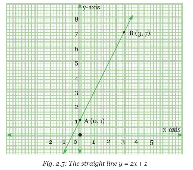
Slope and the Shape of a Line
Slope — In , the coefficient is the slope; it indicates the line's direction and steepness.
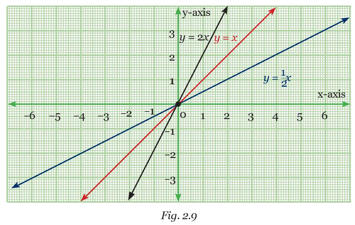
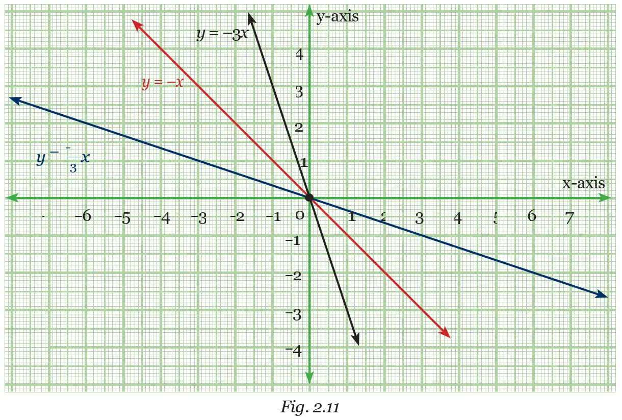
All lines pass through the origin. For positive , the line rises from left to right; for negative , it falls. For positive slopes, values greater than give a steeper line than , while values between and give a less steep line.
Comparing slopes
- Positive slope: A line with positive slope represents linear growth; a line with negative slope represents linear decay.
- Positive lines: In , is steeper than , while is less steep.
- Negative lines: For with , the line falls. The line is steeper than , while is less steep.
- Examples: The points satisfy ; the points satisfy .
- Constant difference: The sequence increases by each time. Its term-number relationship is , so its slope equals the constant difference .
For , the slope is and the graph passes through .
Graphing a line through the origin
- Use the origin as one point.
- Choose a convenient non-zero value of and calculate .
- Plot both points and draw the straight line through them.
Draw the graph of using two points.
- The line passes through the origin.
- Choose another convenient value and calculate its image.
- Plot the points and join them; the negative slope means the line falls from left to right.
| Point | ||
|---|---|---|
| Slope | (rising) | (falling) |
| Y-intercept |
Slope and Y-Intercept in
Y-intercept — The y-intercept is the y-coordinate where a line crosses the y-axis; in , it is and the crossing point is .
In , changing changes the slope while keeping fixed. Changing while keeping fixed shifts the line; lines with equal slopes and different y-intercepts are parallel.
| Line | Y-axis crossing | Y-intercept |
|---|---|---|
Read the slope and y-intercept directly from this form.
Graphing from slope-intercept form
- Plot the y-intercept on the y-axis.
- Choose another convenient -value and calculate .
- Plot the second point and draw the line through both points.
Graph and state its slope and y-intercept.
- Identify the slope and y-intercept.
- Plot the y-intercept.
- Find a second point by substituting .
- Draw the straight line through the two points.
Equal slopes and parallel lines
- Same slope, different intercept: , , and are parallel.
- Different slopes: , , and cut the y-axis at , , and respectively.
Do not confuse slope with y-intercept: in , is the slope and gives the crossing point .
Check whether lies on .
For , state the slope and y-intercept. Is it parallel to ?
Compare the graphs of , , and .
Quick recap
- Plot a linear equation by finding two points that satisfy it and joining them with a straight line.
- For , the line passes through and its slope is .
- Positive slope represents growth; negative slope represents decay.
- For with , larger values of give steeper lines.
- In , is the slope and is the y-intercept at .
- Changing only the y-intercept shifts a line; lines with equal slopes and different intercepts are parallel.
Summary
Algebraic Expressions and Polynomials
Use the highest power with a non-zero coefficient.
Identify a Polynomial's Degree and Type
- Check that the expression is in one variable.
- Find the greatest exponent whose coefficient is non-zero.
- If the degree is , classify it as a linear polynomial.
For , identify its terms, coefficients, and degree.
- For , identify the terms and coefficients.
- The greatest exponent of is .
- Therefore, it is a univariate polynomial of degree , not a linear polynomial.
Classify and state its degree.
Linear Patterns: Growth and Decay
A linear pattern has the same difference between each pair of consecutive terms.
Classify a Linear Pattern
- Subtract each term from the next term.
- Check whether all the differences are equal.
- A positive difference means growth; a negative difference means decay.
Classify the pattern .
- Find the differences in the sequence .
- The differences are constant and positive, so the sequence shows linear growth.
Does the sequence show linear growth or decay?
Linear Relationships and Parallel Lines
Use this form to identify the slope and -intercept directly.
Distinct parallel lines have matching slopes and different intercepts.
Read a Line's Slope and Intercept
- Write the equation in the form .
- Read the coefficient of as the slope and the constant as the -intercept.
- Compare slopes to test whether two lines are parallel.
Determine whether and are parallel.
- In , the slope is and the -intercept is .
- In , the slope is also , but the intercept is .
- Since the slopes match and the intercepts differ, the lines are parallel.
For , state the slope, -intercept, and whether the line shows growth or decay.
Quick recap
- An algebraic expression has terms made from numbers, variables, and operations; coefficients are their numerical factors.
- A univariate polynomial has one variable, and its degree is its greatest exponent with a non-zero coefficient.
- A linear polynomial has degree .
- A linear pattern has a constant difference: positive for growth and negative for decay.
- In , is the slope and is the -intercept; setting gives a line through the origin.
- Lines with the same slope and different -intercepts are parallel.
Formula sheet
Mathematics — ALL CHAPTERS
1
Orienting Yourself: The Use of Coordinates
2
Introduction to Linear Polynomials
3
The World of Numbers
4
Exploring Algebraic Identities
5
I’m Up and Down, and Round and Round
6
Measuring Space: Perimeter and Area
7
The Mathematics of Maybe: Introduction to Probability
8
Predicting What Comes Next: Exploring Sequences and Progression