Class 12 Commerce . Economics . Introductory Macro Economics . Determination of Income and Employment
Chapter 4: Determination of Income and Employment
Ch 4
Economics
Class 12 Commerce
Introduction
Macroeconomic Models and Ceteris Paribus
Why Macroeconomic Models Are Used
- Macroeconomic models are theoretical tools that explain how variables such as national income, the price level and the rate of interest are determined.
- Purpose: Models help explain slow growth, recessions, increases in the price level and rising unemployment.
- Focus: Since analysing all variables together is difficult, a model often studies one variable while holding others constant.
Ceteris paribus — The assumption that other things remain equal while studying the effect of a particular factor.
How a Model Isolates Variables
- Express one variable in terms of another using one relationship.
- Substitute that expression into a second relationship to solve for the variables.
- Macroeconomic analysis applies this approach to study how economic variables are determined.
Framework of This Chapter
- Focus: The chapter explains the determination of national income.
- Assumptions: Prices of final goods are fixed, and the economy’s rate of interest is constant.
- Theoretical basis: The model is based on the theory of John Maynard Keynes.
Aggregate Demand: Planned and Actual Values
Two Meanings of Economic Variables
- Consumption, investment and output may refer to what actually occurred or what people planned to do.
- GDP is the total output of final goods and services in an economy.
- Accounting use: Actual values measured from economic activity during a given year are ex post measures.
- Aggregate-demand analysis: Planned consumption, investment and output are important for explaining how income is determined; these are ex ante measures.
| Point | Ex ante | Ex post |
|---|---|---|
| Meaning | Planned or intended value | Actual value that occurred |
| Investment example | Amount a producer plans to add to inventory | Amount inventory actually increases by |
Planned and Actual Investment Example
- Plan: A producer intends to add goods worth Rs. 100 to inventory.
- Unexpected sales: Extra demand leads the producer to sell Rs. 30 worth of goods from inventory.
- Result: Planned investment is Rs. 100, but the actual increase in inventory is Rs. 70.
Actual inventory increase equals the planned addition minus goods sold from stock.
- Macroeconomic model
- A theoretical tool for explaining how economic variables are determined.
- Ceteris paribus
- The assumption that other things remain equal.
- Ex ante
- A planned or intended value.
- Ex post
- An actual value measured after events have occurred.
Quick recap
- Macroeconomic models explain how key economic variables are determined.
- Ceteris paribus means studying a factor while holding other things constant.
- This chapter assumes fixed prices of final goods and a constant rate of interest.
- The chapter’s theoretical model is based on Keynesian theory.
- GDP is the total output of final goods and services in an economy.
- Ex ante values are planned; ex post values are actual.
- Unexpected sales can make actual investment differ from planned investment.
Consumption
Consumption Function
Consumption function — A consumption function shows how household consumption expenditure changes with income.
- Main determinant: Household income is the most important determinant of consumption demand.
- Autonomous consumption: Consumption independent of income; it may occur even when income is zero.
- Induced consumption: The part of consumption that varies with income.
- Total consumption: It consists of autonomous and induced consumption.
Here, is consumption expenditure, is autonomous consumption, is induced consumption, and is the marginal propensity to consume.
In Imagenia, autonomous consumption is Rs. 100. For every Rs. 100 increase in income, consumption rises by Rs. 80.
Marginal Propensity to Consume (MPC)
Marginal propensity to consume (MPC) — MPC is the change in consumption per unit change in income; it is denoted by .
It measures the rate at which consumption changes as income changes.
Possible values of MPC
- Range: , because the change in consumption cannot exceed the change in income.
- If : Consumption does not change when income changes.
- If : The entire change in income is spent on consumption.
- If : Part of the change in income is spent on consumption.
Saving and Marginal Propensity to Save (MPS)
Saving — Saving is the part of income that is not consumed.
Income is divided between consumption and saving.
Marginal propensity to save (MPS) — MPS is the change in saving per unit change in income; it is denoted by .
Since income is allocated to consumption or saving, the marginal propensities add up to one.
The marginal propensities to consume and save together account for the whole change in income.
Average Propensities
Average propensity to consume (APC) — APC is consumption per unit of income.
Average propensity to save (APS) — APS is saving per unit of income.
State the relationship between MPC and MPS.
Quick recap
- The consumption function relates household consumption to income: .
- Autonomous consumption is independent of income; induced consumption varies with income.
- MPC measures the change in consumption per unit change in income: .
- MPC lies between zero and one, inclusive.
- Saving is income not consumed: .
- MPS measures the change in saving per unit change in income, and .
- APC is ; APS is .
Investment
Investment
is a positive constant: investment is assumed to be independent of current income in this model.
Two-Sector Equilibrium
In an economy without government, planned aggregate demand equals planned consumption plus planned investment. Equilibrium requires planned output to equal planned demand.
Reading the Equilibrium Equation
- Autonomous expenditure: combines autonomous consumption and investment.
- Consumption: Planned consumption has an autonomous part, , plus income-related consumption, .
- Fluctuations: Autonomous consumption is relatively stable, while investment can fluctuate periodically.
- Equilibrium condition: holds when planned output and planned aggregate demand are equal.
| Point | Ex ante | Ex post |
|---|---|---|
| Meaning | Planned output, consumption, investment or demand. | Actual output, consumption and investment after production and sales. |
| Equality | Planned output equals planned demand only in goods-market equilibrium. | Actual output always equals actual consumption plus actual investment; unsold goods count as inventory investment. |
| Inventory effect | If planned demand falls short of planned output, firms accumulate unintended stocks. | The extra unsold output appears as inventory investment in the accounting identity. |
Inventory Investment
- Inventory: Output produced but not sold, and therefore still held by the firm.
- Positive investment: Inventory rises as unsold stocks accumulate.
- Negative investment: Inventory falls as existing stocks are depleted.
- Planned inventory investment: A deliberate decision by a firm to hold stocks.
- Unplanned inventory investment: A change in stocks because actual sales differ from planned sales.
Do not treat as an identity for planned values: it is the equilibrium condition for ex ante values. The ex post identity includes actual inventory investment, including unintended changes in stocks.
Introducing Government
Government expenditure on final goods adds to demand. Taxes reduce household disposable income, of which households spend a fraction on consumption.
Government and Income
- Fiscal variables: Government expenditure, , and taxes, , are treated as autonomous.
- Disposable income: is the income households have after taxes.
- Autonomous demand: Government shifts the autonomous part of demand by ; it does not change the basic analysis qualitatively.
- Scope: The chapter then ignores government for simplicity. Without indirect taxes and subsidies, GDP equals National Income, so is used for either.
Quick recap
- Investment adds to physical capital or changes producers’ inventories; here, planned investment is autonomous: .
- In the two-sector model, and equilibrium requires planned output to equal planned demand.
- Autonomous expenditure is , giving the equilibrium relation .
- Inventory investment is positive when stocks rise and negative when stocks fall; it may be planned or unplanned.
- The ex post identity includes actual inventory changes, while ex ante output equals demand only in equilibrium.
- With government, disposable income is and equilibrium demand includes ; without indirect taxes and subsidies, GDP equals National Income.
Determination Of Equilibrium Income In The Short Run
Short-Run Macroeconomic Equilibrium
Why begin with a fixed price level?
- Two-stage analysis: First determine macroeconomic equilibrium with the price level fixed; later, allow the price level to change.
- Unused resources: With idle machinery, buildings and labour, extra output can be produced without raising marginal cost, so the price level need not rise.
- Simplification: Treating prices as fixed is also a simplifying assumption for the first stage of analysis.
Macroeconomic Equilibrium with a Fixed Price Level
- Equilibrium: In the final goods market, equilibrium occurs when planned aggregate demand equals planned output, so there is no unintended change in inventories.
- Equilibrium income: In the two-sector model, income is determined by autonomous expenditure and the marginal propensity to consume: .
Graphical Method
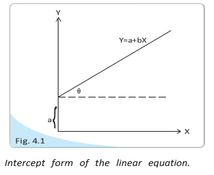
Intercept form — A linear relation written as , where is the vertical intercept and is the slope.
- Intercept: is the value of when .
- Slope: measures the change in for a unit change in ; graphically, .
Consumption Function
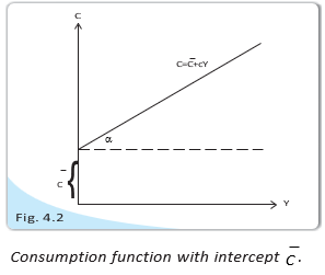
Autonomous consumption plus consumption that varies with income.
- Autonomous consumption (): Consumption when income is zero; it is the vertical intercept.
- Marginal propensity to consume (): The slope of the consumption function; graphically, .
- Shape: Consumption rises with income, beginning at the positive intercept .
Investment Function
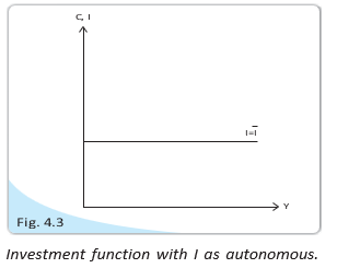
In the two-sector model, investment is constant at every income level.
- Graph: A horizontal line at the level , because investment does not change as income changes.
Aggregate Demand
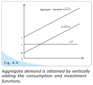
Aggregate demand — The total planned demand for final goods and services at each income level; in this two-sector model it is consumption plus investment.
Adding autonomous investment to consumption gives the aggregate demand function.
- Graphical construction: Add consumption and investment vertically at each income level.
- Slope: The aggregate demand line is parallel to the consumption line because both have slope .
- Ex ante demand: Aggregate demand represents planned expenditure.
Aggregate Supply
- Fixed-price assumption: With unused resources available, output can adjust to meet demand without changing the price level.
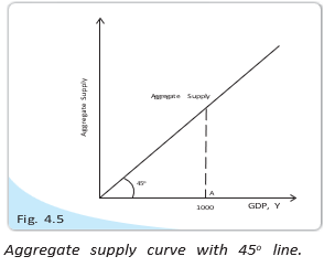
- 45° line: Aggregate supply is represented by a line where output/income equals aggregate supply; every point has equal horizontal and vertical coordinates.
- Meaning: If income/output is Rs. 1,000, the corresponding supply is also Rs. 1,000.
Equilibrium: Graphical Method
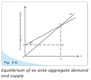
Equilibrium income — The income level at which planned (ex ante) aggregate demand equals planned aggregate supply.
- Graphical condition: Equilibrium is where the ex ante aggregate demand curve intersects the 45° aggregate supply line.
- Equilibrium point: The intersection is marked ; its corresponding income is .
Algebraic Method
Equilibrium requires planned aggregate demand to equal aggregate supply.
Solve the equilibrium condition for income.
- Interpretation: Equilibrium income depends on autonomous consumption and investment, divided by .
- Symbols: is income/output; is autonomous consumption; is autonomous investment; is the marginal propensity to consume.
Do not omit autonomous investment or use as the denominator: equilibrium income is .
State the equilibrium condition and the formula for equilibrium income.
Why is aggregate supply shown as a 45° line in the fixed-price model?
Quick recap
- Short-run analysis first holds the price level fixed, partly because unused resources permit more output without higher marginal cost.
- The consumption function is ; is its intercept and its slope.
- Investment is autonomous: , represented by a horizontal line.
- Aggregate demand is and is planned (ex ante) demand.
- Aggregate supply is represented by the 45° line, where supply equals income/output.
- Equilibrium occurs where ex ante aggregate demand equals aggregate supply.
- Equilibrium income is .
Effect of an Autonomous Change in Aggregate Demand on Income and Output
Changes in Aggregate Demand
- Sources of change: Aggregate demand can change because of changes in consumption or investment.
- Income and output: A change in aggregate demand shifts the equilibrium level of income and output; the multiplier can make the total change larger than the initial change in autonomous expenditure.
An Increase in Autonomous Investment
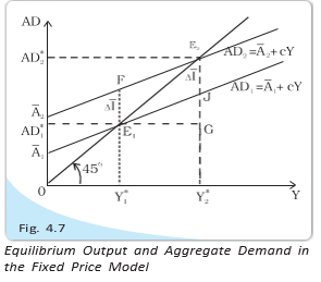
The Multiplier Mechanism
The repeated increases form an infinite geometric series. For an initial autonomous increase of and , total output rises by .
Investment Multiplier
Here, is the total change in equilibrium output and is the initial change in autonomous expenditure.
Why does a change in autonomous expenditure cause a larger change in equilibrium output?
If and autonomous expenditure rises by , find the multiplier and the total increase in equilibrium output.
Quick recap
- Equilibrium income occurs where .
- Changes in consumption or autonomous investment can change aggregate demand and equilibrium income.
- An increase in autonomous expenditure creates successive rounds of induced consumption and output.
- With , an autonomous spending increase of raises equilibrium output by .
- The investment multiplier is ; a higher means a larger multiplier.
Paradox of Thrift
The paradox of thrift
Paradox of thrift — When everyone tries to save a larger proportion of income, total saving may remain unchanged or fall because lower consumption reduces income.
Key idea
- Thrift means a greater willingness to save; in the model, higher MPS corresponds to lower MPC.
- Aggregate effect: reduced consumption lowers aggregate demand, output and income through successive rounds.
- Result: people intend to save more, but the economy-wide total saving can remain unchanged or decline.
In the simple income-determination model, equilibrium output equals aggregate demand; is autonomous expenditure and is MPC.
How greater thrift changes income and saving
Adjustment in successive rounds
- Initial equilibrium: with and , output is .
- Behavioural change: an external event, such as fear of an impending disaster, may make households more cautious; MPC falls from to .
- First demand fall: at income , consumption and aggregate demand fall by .
- Output adjustment: excess supply prompts producers to reduce output and income; each later round reduces demand by half the previous round.
- Total output fall: reductions form the convergent series .
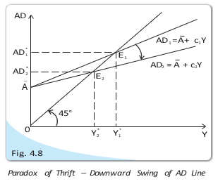
Aggregate-demand line
- Change in autonomous expenditure: changing shifts the aggregate-demand line up or down in parallel.
- Change in MPC: changing changes the line's slope; a fall in MPC makes it less steep and swings it downward.
| Situation | MPC | Equilibrium output | Aggregate saving |
|---|---|---|---|
| Initial | |||
| After thrift rises |
- Example result: output falls by , from to , while aggregate saving remains .
- Why saving stays unchanged: lower MPC reduces equilibrium income, offsetting the greater intended propensity to save.
Equilibrium and full employment
Full-employment income — The level of income at which all factors of production are fully employed.
Equilibrium does not guarantee full employment
- Output and employment: equilibrium output helps determine employment when the quantities of other factors of production are given.
- Equilibrium condition: means income will not change on its own; it does not mean that all resources are employed.
- Possible gap: equilibrium output may be below or above full-employment output.
| Point | Deficient demand | Excess demand |
|---|---|---|
| Output relative to full employment | Equilibrium output is below full-employment output. | Equilibrium output is above full-employment output. |
| Cause | Demand is insufficient to employ all factors of production. | Demand exceeds the output produced at full employment. |
| Long-run price effect | Prices tend to fall. | Prices tend to rise. |
What is the paradox of thrift?
Distinguish deficient demand from excess demand.
Quick recap
- Higher thrift means higher MPS and lower MPC.
- Lower MPC reduces aggregate demand and equilibrium income through successive rounds.
- In the example, MPC falls from to and output falls from to .
- Aggregate saving remains in both equilibria: this is the paradox of thrift.
- Equilibrium at does not guarantee full employment.
- Deficient demand tends to lower prices; excess demand tends to raise prices in the long run.
Summary & Key Concepts
Aggregate Demand and Equilibrium
Aggregate demand (AD) — The total planned expenditure on final goods in an economy at a given price level.
Components and equilibrium
- Components: Aggregate demand includes ex ante consumption, ex ante investment, government spending and other planned expenditure.
- Product-market equilibrium: At a particular price level, equilibrium occurs when aggregate demand for final goods equals their aggregate supply.
Equilibrium occurs when aggregate demand equals aggregate supply.
Ex Ante, Ex Post and Inventory Changes
| Point | Ex Ante | Ex Post |
|---|---|---|
| Meaning | Planned or intended spending, saving or production | Actually realised spending, saving or production |
| Use in equilibrium | Planned aggregate demand is compared with output | Realised outcomes may differ from plans |
Unintended changes in inventories
- Unintended inventory changes: These occur when actual sales differ from planned sales, causing firms’ inventories to accumulate or run down unexpectedly.
Consumption and Marginal Propensity to Consume
Marginal propensity to consume (MPC) — The increase in ex ante consumption caused by a unit increase in income.
It measures the change in planned consumption relative to the change in income.
Aggregate Supply and Effective Demand
Aggregate supply (AS) — The total output of final goods supplied by producers in the economy.
Short-run assumptions and output
- Assumptions: In the short run, the final-goods price level and interest rate are constant; aggregate supply is perfectly elastic at that price.
- Implication: Under these assumptions, aggregate output is determined by aggregate demand.
- Effective demand principle: The level of aggregate demand determines aggregate output in the economy.
Autonomous Spending and the Multiplier
Autonomous expenditure — Expenditure that does not change directly with current income.
Autonomous change
- Autonomous change: Listed as a key concept in this lecture summary; no further explanation is provided there.
Autonomous expenditure multiplier — The factor describing how an autonomous expenditure change leads to a larger change in aggregate output through the multiplier process.
Multiplier process
- Autonomous spending rises → aggregate demand rises.
- Higher aggregate demand increases output.
- An increase in output and income induces further consumption, raising aggregate demand again.
- The resulting total output change is larger than the initial autonomous spending change.
Direction of the multiplier effect
- Increase: An increase in autonomous spending raises aggregate output by a larger amount through the multiplier process.
- Decrease: A decrease in autonomous spending lowers aggregate output by a larger amount through the multiplier process.
Other Key Concepts
Terms listed in the lecture summary
- Parametric shift and paradox of thrift are listed as key concepts; this summary does not explain them.
State the effective demand principle.
Why can a change in autonomous spending cause a larger change in output?
Quick recap
- Product-market equilibrium occurs when aggregate demand equals aggregate supply.
- Ex ante means planned; ex post refers to realised outcomes.
- MPC is the increase in ex ante consumption caused by a unit increase in income.
- With fixed prices and interest rates and perfectly elastic aggregate supply, demand determines output.
- An autonomous spending change can produce a larger output change through the multiplier process.
- Parametric shift, unintended inventory changes and paradox of thrift are listed as key concepts in the summary.
Economics — ALL CHAPTERS
1
Indian Economy On The Eve Of Independence
2
Indian Economy 1950–1990
3
Liberalisation, Privatisation And Globalisation: An Appraisal
4
Human Capital Formation In India
5
Rural Development
6
Employment : Growth, Informalisation And Other Issues
7
Environment and Sustainable Development
8
Comparative Development Experiences of India And Its Neighbours
1
Introduction
2
National Income Accounting
3
Money and Banking
4
Determination of Income and Employment
5
Government Budget and the Economy
6
Open Economy Macroeconomics