Class 11 PCM . Physics . Physics Part I . Motion in a Plane
Chapter 3: MOTION IN A PLANE
Ch 3
Physics
Class 11 PCM
Introduction
Why Vectors Are Needed
Scope of the chapter
- One dimension: Direction can be shown using positive and negative signs because motion has only two possible directions along a line.
- Two or three dimensions: Position, displacement, velocity and acceleration need vectors to represent direction as well as magnitude.
- Topics ahead: Vector operations, motion with constant acceleration, projectile motion and uniform circular motion.
- Extension: The equations for motion in a plane can be extended to three dimensions.
Scalars and Vectors
| Type | Definition | Examples | Combining quantities |
|---|---|---|---|
| Scalar | Has magnitude only; a number and its unit specify it fully. | Distance, mass, temperature and time. | Use ordinary algebra; addition or subtraction requires the same units. |
| Vector | Has both magnitude and direction, and obeys the triangle law (equivalently, the parallelogram law) of addition. | Displacement, velocity, acceleration and force. | Direction must be accounted for when combining vectors. |
Scalar examples and notation
- Perimeter: A rectangle of length and breadth has perimeter ; both length and perimeter are scalars.
- Temperature difference: .
- Density example: A cube of side and mass has volume and density .
- Vector notation: A vector may be written in bold, such as , or by hand with an arrow, such as .
- Magnitude: The magnitude (absolute value) of is written ; the vector is bold and its magnitude is light-face.
Position and Displacement Vectors
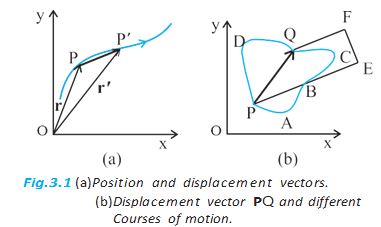
Position vector — The vector from a chosen origin to an object's position gives its position relative to that origin.
Describing position and motion
- At time : If the object is at , its position vector is .
- At time : If it moves to , its position vector is .
- Displacement: The vector points from the initial position to the final position .
- Path independence: Displacement depends only on the initial and final positions, not on the route taken between them.
- Magnitude: The magnitude of displacement is less than or equal to the path length between the two positions.
Equality of Vectors
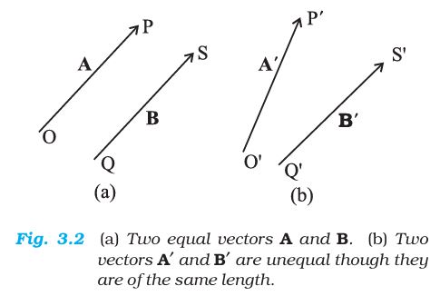
Equal vectors — Vectors and are equal if and only if they have the same magnitude and the same direction.
How to check equality
- Translation: A vector may be shifted parallel to itself without changing it; compare the vectors after bringing their tails together.
- Equal vectors: If their tips then coincide, the vectors are equal, written .
- Direction matters: Vectors with the same magnitude but different directions are not equal.
- Free vectors: In this study, vectors have no fixed location, so parallel shifting leaves them unchanged.
- Localised vectors: In some applications, a vector's location or line of application matters.
When are two vectors equal?
Does displacement depend on the path taken?
Quick recap
- Scalars have magnitude only; vectors have magnitude and direction.
- Scalar addition and subtraction require quantities with the same units.
- A position vector runs from the chosen origin to the object's position.
- Displacement depends only on the start and end positions, not the route.
- Equal vectors have the same magnitude and direction, regardless of location.
- Free vectors can be shifted parallel to themselves; localised vectors depend on location or line of application.
Multiplication Of Vectors By Real Numbers
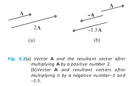
Multiplication of a Vector by a Scalar
Vector Addition: Head-to-Tail Method
Laws of Vector Addition
Null Vector
Vector Subtraction
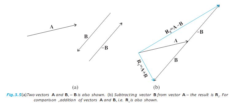
Parallelogram Method
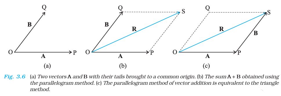
How can vector subtraction be expressed as vector addition?
State the commutative and associative laws of vector addition.
Quick recap
- A positive scalar changes a vector’s magnitude but not its direction; a negative scalar also reverses its direction.
- A dimensioned scalar multiplies the vector’s dimensions; velocity times duration gives displacement.
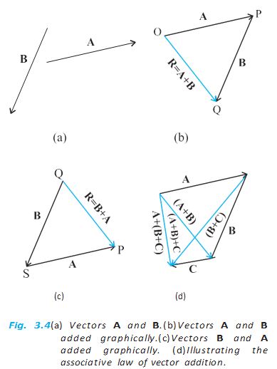
- Head-to-tail addition and the triangle method produce the resultant from the first tail to the last head.
- Vector addition is commutative and associative.
- A null vector has zero magnitude and no specified direction; it represents zero net displacement.
- Subtraction means adding the negative vector; the parallelogram diagonal gives the same resultant as the triangle method.
Resolution Of Vectors
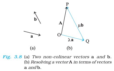
Resolution Along Two Directions
Unit Vectors
Each coordinate-axis unit vector has magnitude one.
Here is a unit vector along .
Components in Two Dimensions
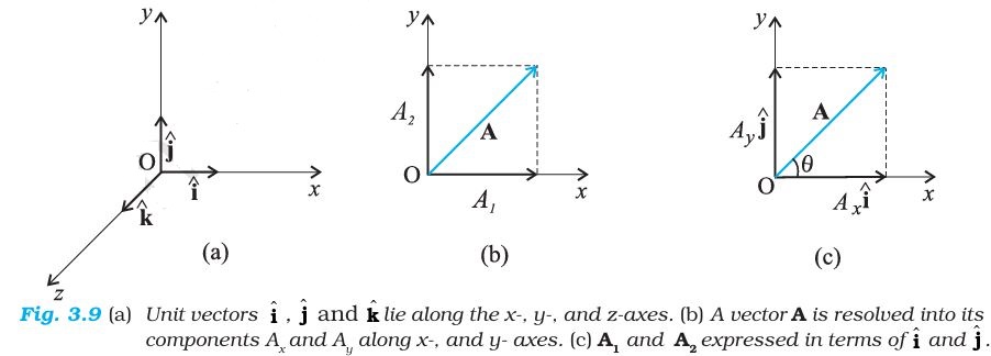
If is measured from the positive -axis, use these relations to find the components.
Use the perpendicular components to find the vector’s magnitude.
The angle is measured from the positive -axis; use the component signs to select the correct quadrant.
Do not treat or as vectors: they are scalar components; the corresponding vectors include the unit vectors.
Components in Three Dimensions
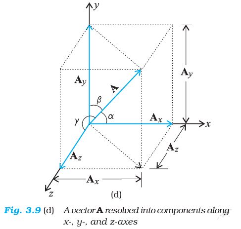
The direction cosines give the components along each axis.
Use the three mutually perpendicular components to find the magnitude.
Position Vector
Quick recap
- Resolve a planar vector as a sum of components along two non-parallel directions.
- Unit vectors have magnitude one and specify direction; the coordinate unit vectors are mutually perpendicular.
- In two dimensions, .
- Find 2D components with and ; recover magnitude using Pythagoras.
- In three dimensions, the component values use direction cosines and the vector is the sum of its three axis components.
- A position vector is written as .
Vector Addition- Analytical Method
Adding vectors by components
A vector in the - plane is written using its components along the unit vectors and .
For , add the -components together and the -components together.
Extension to three dimensions and multiple vectors
In three dimensions, add corresponding components along the , and axes.
Add or subtract the components on each axis using the same signs as the vector expression.
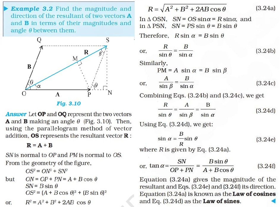
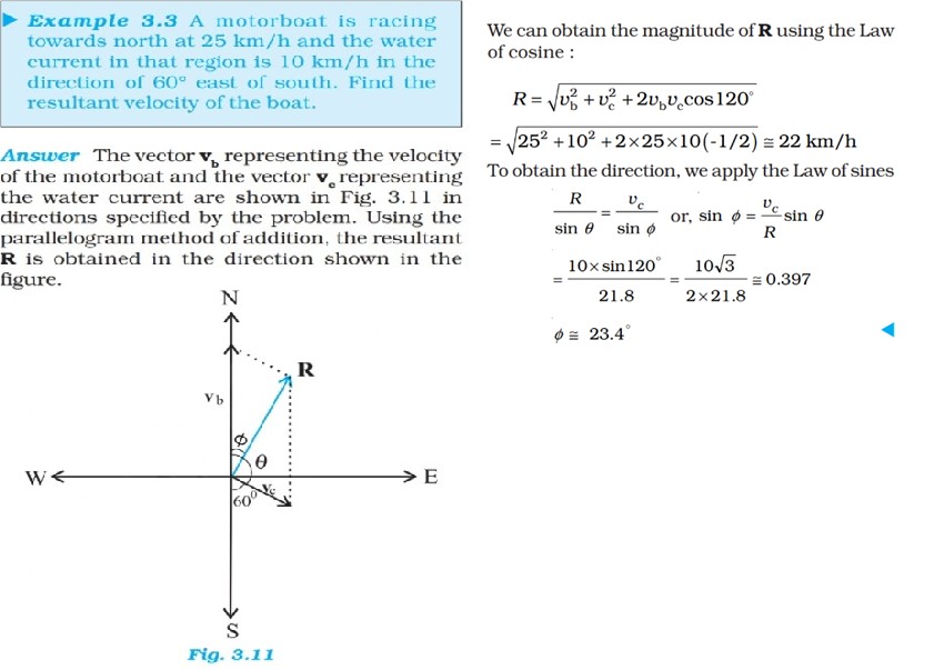
Do not add vector magnitudes directly unless the vectors point along the same line and direction; add corresponding signed components instead.
How are two vectors added analytically in two dimensions?
Quick recap
- Analytical addition combines vectors through their components.
- In two dimensions, add the -components and -components separately.
- In three dimensions, add corresponding , and components.
- For multiple vectors, keep the signs from the vector expression when combining components.
Motion In A Plane
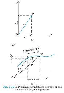
Position Vector and Displacement
Position vector — The position vector gives a particle’s location relative to the origin of the coordinate frame.
For coordinates and , the position vector is:
- Components: and are the particle’s coordinates along the - and -axes.
- Displacement: The change in position from to is ; it points from the initial to the final position.
- Components of displacement: and , so .
Velocity
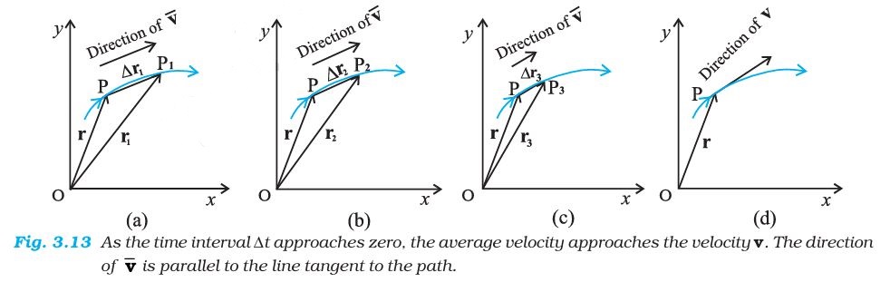
Average velocity — Average velocity is the displacement divided by the time interval over which it occurs.
Its direction is the same as the displacement direction.
Instantaneous velocity — Instantaneous velocity is the limiting value of average velocity as the time interval approaches zero.
The velocity vector is tangent to the path and points in the direction of motion.
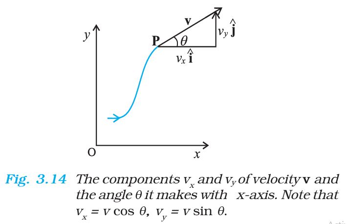
- Components: If position coordinates are known as functions of time, differentiate each coordinate to obtain the corresponding velocity component.
- Magnitude: The speed is the magnitude of the velocity vector.
- Direction: The angle is measured from the positive -axis.
The coordinate derivatives give the vector components.
Use the component ratios to find the angle with the -axis.
Acceleration
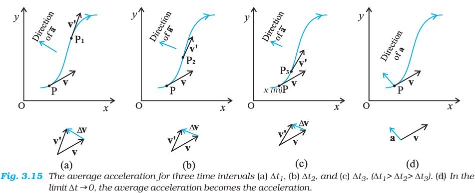
Average acceleration — Average acceleration is the change in velocity divided by the time interval.
Its direction is the same as the change in velocity, .
Instantaneous acceleration — Instantaneous acceleration is the limiting value of average acceleration as the time interval approaches zero.
Acceleration components are the time derivatives of the velocity components.
- Direction in 1D: Velocity and acceleration lie along the same straight line; they can point in the same or opposite directions.
- Direction in 2D or 3D: Velocity and acceleration can form any angle from to .
Worked Example: Position to Velocity and Acceleration
Given and results
- Position: , with position in metres and in seconds.
- Differentiate position: ; the constant -component gives zero velocity in that direction.
- Differentiate velocity: , so acceleration has magnitude along the -direction.
- At : .
- Magnitude and direction: and to the -axis.
Do not confuse speed with velocity: speed is the magnitude of velocity, while velocity also has direction.
Quick recap
- Position: locates a particle relative to the origin.
- Displacement: points from the initial to the final position.
- Velocity: Average velocity is ; instantaneous velocity is and is tangent to the path.
- Velocity components: and ; magnitude is .
- Acceleration: Average acceleration is ; instantaneous acceleration is .
- Components: and ; in multidimensional motion, acceleration need not align with velocity.
Motion In A Plane With Constant Acceleration
Velocity under Constant Acceleration
Constant acceleration — Acceleration remains unchanged with time; therefore, average acceleration over any interval equals this constant value.
Use when acceleration is constant over the time interval.
Apply the relation separately in the two perpendicular directions.
Position under Constant Acceleration
Displacement from Average Velocity
- Average velocity: With constant acceleration, the average velocity from to is .
- Displacement: Multiply the average velocity by the elapsed time: .
- Position: Add this displacement to the initial position vector.
The position at time for constant acceleration.
Use these equations to find each coordinate independently.
Independent Motion in Perpendicular Directions
- Independence: Motion in the - and -directions can be treated as two simultaneous one-dimensional motions.
- Shared time: Both directions use the same elapsed time, although their velocities and accelerations may differ.
- Extension: The same independent-component treatment applies in three dimensions.
Do not use separate elapsed times for the two directions: both coordinate equations describe the particle at the same instant.
Example: Coordinate and Speed
- Given: A particle starts at the origin with and .
- Position: and ; setting gives .
- Coordinate: At this time, .
- Velocity: , so at , .
- Speed: .
Quick recap
- For constant acceleration, .
- Position follows .
- Apply the velocity and position relations separately to the - and -components.
- The two component motions are independent but occur over the same time interval.
- Speed is the magnitude of velocity: .
Projectile Motion
Projectile motion and its components
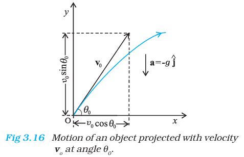
Equations of projectile motion
Use these components for a projectile launched from the origin.
These equations apply when the launch point is the origin.
Motion at the highest point
- At the apex: The vertical velocity is zero, , while the horizontal velocity remains .
- Direction: At the apex, the velocity is horizontal.
Path of a projectile
Trajectory — The trajectory is the path followed by the projectile; eliminating time gives a parabola.
Since this has the form , the projectile's path is parabolic.
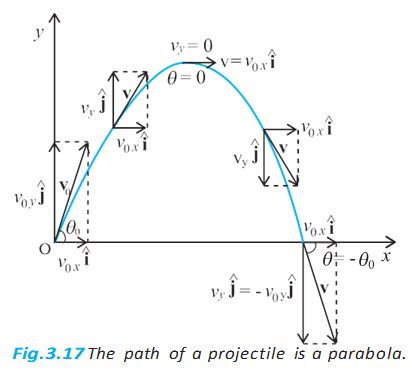
Maximum height and time of flight
At the maximum height, set .
For launch and landing at the same height, the total flight time is twice the time to maximum height.
The maximum vertical displacement above the launch level.
Horizontal range
Horizontal range — The horizontal distance from launch point to the landing point at the same vertical level.
Range equals horizontal speed multiplied by time of flight.
Range facts
- Maximum range: For fixed , the range is greatest at , giving .
- Complementary angles: Launch angles and give equal ranges because their doubled angles have equal sine.
Worked applications
Horizontal throw from a cliff
- Given: A stone is thrown horizontally at from a cliff; take .
- Fall time: Vertical motion gives , so .
- Impact speed: and ; hence speed .
Oblique throw returning to launch level
- Given: A ball is thrown at and above the horizontal; use .
- Results: , , and .
Quick recap
- Projectile motion combines uniform horizontal motion with vertically accelerated motion under gravity.
- Resolve the initial velocity into and .
- The trajectory is parabolic; at its highest point, .
- For equal launch and landing heights, and .
- The range is and is maximum at .
- Complementary launch angles have equal ranges when launch and landing heights are the same.
Uniform Circular Motion
Meaning and Direction of Acceleration
Uniform circular motion — Motion along a circular path at constant speed.
- Constant speed, changing velocity: Velocity changes continuously because its direction changes, so the object is accelerated even though its speed is constant.
- Velocity direction: At every point, velocity is tangent to the circle and perpendicular to the radius.
- Acceleration direction: The change in velocity, and hence acceleration, points towards the centre of the circle.
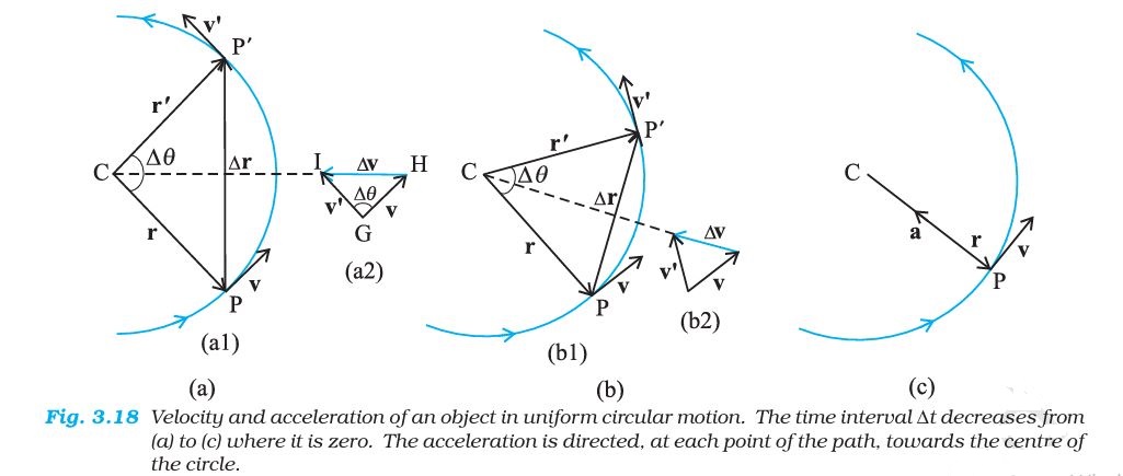
Centripetal Acceleration
- Centripetal acceleration: Acceleration in circular motion is always directed towards the centre; “centripetal” means centre-seeking.
- Magnitude: Similar triangles formed by the radii and velocity vectors give the acceleration magnitude in terms of speed and radius.
- Direction vs magnitude: Its magnitude stays constant when speed and radius are constant, but its direction continuously changes; therefore, acceleration is not a constant vector.
The instantaneous acceleration is the limit of average acceleration as the time interval approaches zero.
Use for an object moving at speed in a circle of radius .
Angular Speed and Linear Speed
Angular speed — The rate of change of angular displacement; for a time interval, .
- Angular displacement: The angle swept by the radius as the object moves.
- Arc length: For angular displacement measured in radians, the distance travelled along the circle is .
- Speed relation: Dividing arc length by time gives .
Relates tangential speed and angular speed.
Substitute into .
Time Period and Frequency
Time period — The time taken to complete one revolution, denoted by .
Frequency — The number of revolutions completed per second, denoted by .
- One revolution: The object travels a distance and sweeps an angle radians.
- Frequency and period: They are reciprocals: and .
Equivalent forms using the number of revolutions per second.
Example: Insect in a Circular Groove
Given: radius ; revolutions in
- Angular speed: .
- Linear speed: .
- Acceleration magnitude: .
- Vector behaviour: Acceleration points towards the centre, so its direction changes continuously; its magnitude remains constant.
Constant speed does not mean constant velocity or zero acceleration: velocity direction changes, producing centripetal acceleration.
Why is an object in uniform circular motion accelerated despite having constant speed?
Quick recap
- Uniform circular motion has constant speed but continuously changing velocity.
- Velocity is tangential; centripetal acceleration points towards the centre.
- Instantaneous acceleration magnitude is .
- Centripetal acceleration magnitude is .
- Angular speed is and linear speed is .
- Time period is time per revolution; frequency is revolutions per second, with .
- Frequency forms: , , and ; in the groove example, , , and .
Summary And Points To Ponder
Scalars and Vectors
Scalar quantity — A physical quantity described by magnitude only.
Vector quantity — A physical quantity described by both magnitude and direction; vectors follow the rules of vector algebra.
| Scalars | Vectors | |
|---|---|---|
| Description | Magnitude only | Magnitude and direction |
| Examples | Distance, speed, mass, temperature | Displacement, velocity, acceleration |
Multiplying a Vector by a Scalar
- Magnitude: For real number , the vector has magnitude .
- Direction: It points along if and opposite to if .
Vector Operations and Components
Vector Addition and Subtraction
- Addition: Add vectors graphically by the head-to-tail or parallelogram method.
- Commutative law: The order of addition does not matter: .
- Associative law: Grouping does not matter: .
- Subtraction: Subtracting means adding its opposite: .
Null (zero) vector — A vector with zero magnitude; its direction is unspecified.
Adding a zero vector leaves a vector unchanged; multiplying it by any scalar, or adding it to itself, gives the zero vector.
Resolving Vectors into Components
- Resolution: A vector in a plane can be written as a linear combination of two given vectors in that plane: , where and are real numbers.
- Unit vector: The unit vector along a non-zero vector is .
- Cartesian unit vectors: , , and point along the positive -, -, and -axes in a right-handed coordinate system.
- Two-dimensional form: ; if it makes angle with the positive -axis, then and .
Use the component magnitudes to find the vector magnitude and its angle from the positive -axis.
Add corresponding components to obtain the resultant of two vectors in the - plane.
Position, Displacement and Motion
The position vector locates an object relative to the origin; displacement is the change in its position.
Average and Instantaneous Velocity
- Average velocity: Displacement divided by the elapsed time: .
- Instantaneous velocity: The limiting value of average velocity as the time interval approaches zero: .
- Components: , where , , and .
- Direction: Instantaneous velocity is tangent to the path at the object's position.
Average acceleration is the velocity change per elapsed time; instantaneous acceleration is the rate of change of velocity.
Motion with Constant Acceleration
- Vector equations: For constant acceleration, initial position and initial velocity specify the motion at time .
- Independent directions: Plane motion can be treated as two simultaneous one-dimensional motions along perpendicular axes.
- Axes: The vector equations do not depend on a particular choice of coordinate axes; they can be resolved along any two independent axes.
Use these equations when the acceleration vector is constant.
Apply the vector equations separately to the and directions.
Projectile Motion
Projectile — An object in flight after being projected.
Projectile Motion Basics
- Initial velocity: If launch speed is at angle to the -axis, its components are horizontally and vertically.
- Acceleration: Gravity acts vertically downward with magnitude ; horizontal velocity stays constant while vertical velocity changes.
- Trajectory: The path is parabolic. The range formula below assumes the projectile returns to its launch height.
For launch from the origin, these equations give position and velocity at time .
Eliminating time gives the parabolic path equation.
At maximum height, the vertical velocity is zero.
Range is the horizontal distance from launch to the point where the projectile returns to .
Uniform Circular Motion
Uniform circular motion — Motion along a circular path at constant speed.
Circular Motion Relationships
- Centripetal acceleration: Its magnitude is and its direction is always toward the circle's centre.
- Angular speed: The rate of change of angular position; it relates to linear speed by .
- Frequency and period: If is frequency and is the period, then .
Equivalent expressions connect angular speed, linear speed, frequency and centripetal acceleration.
| Quantity | Symbol | Dimensions | SI unit | Key relation |
|---|---|---|---|---|
| Position vector | Vector | |||
| Displacement | Vector | |||
| Average velocity | ||||
| Instantaneous velocity | ||||
| Average acceleration | ||||
| Instantaneous acceleration | ||||
| Time to maximum height | ||||
| Maximum height | ||||
| Horizontal range | ||||
| Angular speed | ||||
| Centripetal acceleration |
Points to Ponder
| Path length | Magnitude of displacement | |
|---|---|---|
| Depends on | The actual route travelled | Only the initial and final positions |
| Relationship | Usually greater; equal only if direction does not change | Never greater than path length |
Speed, Velocity and Relative Motion
- Average speed and velocity: Average speed is always greater than or equal to the magnitude of average velocity; equality holds when path length equals displacement magnitude.
- Resultant velocity: For two velocities measured in the same reference frame, .
- Relative velocity: Velocity of object 1 relative to object 2 is ; both velocities must use a common reference frame.
Acceleration and Trajectory
- Uniform circular motion: Constant-acceleration kinematic equations do not apply because acceleration changes direction, even though its magnitude stays constant.
- Circular acceleration: The resultant acceleration points toward the centre only when speed is constant; changing speed adds a tangential component.
- Trajectory: Acceleration alone does not determine the path; initial position and initial velocity also matter.
- Example: Under the same gravitational acceleration, different initial conditions can produce a straight-line path or a parabolic path.
Why is the magnitude of displacement generally less than the path length?
Why do constant-acceleration kinematic equations not apply to uniform circular motion?
What determines an object's trajectory?
Quick recap
- Scalars have magnitude only; vectors have magnitude and direction and obey vector-algebra rules.
- Resolve vectors into components to add them, find their magnitude, and determine their direction.
- Displacement, velocity and acceleration are vector quantities; instantaneous velocity is tangent to the path.
- Constant-acceleration plane motion separates into simultaneous motions along perpendicular axes.
- Projectile motion follows a parabola under gravity; its height, time of rise and range follow the standard formulas.
- Uniform circular motion has inward centripetal acceleration; its vector direction changes continuously.
- Path length is at least displacement magnitude, and trajectory depends on both acceleration and initial conditions.
Physics — ALL CHAPTERS
1
Units And Measurement
2
MOTION IN A STRAIGHT LINE
3
MOTION IN A PLANE
4
LAWS OF MOTION
5
WORK, ENERGY AND POWER
6
SYSTEMS OF PARTICLES AND ROTATIONAL MOTION
7
GRAVITATION
8
Mechanical Properties Of Solids
9
Mechanical Properties Of Fluids
10
Thermal Properties Of Matter
11
Thermodynamics
12
Kinetic Theory
13
Oscillations
14
Waves