Calculus — Calculus is the branch of mathematics that studies how a function’s value changes as points in its domain change.
Intuitive Idea of Derivatives
Definition
Derivative — A derivative represents the instantaneous rate at which a function’s value changes with respect to its input.
Falling body: distance and velocity
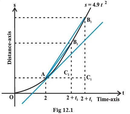
Distance function: A body dropped from a tall cliff travels a distance given by s=4.9t2, where s is in metres and t is in seconds.
Average velocity over an interval is the change in distance divided by the change in time.
Instantaneous velocity at a particular time is estimated using average velocities over increasingly short intervals near that time.
Derivative meaning: For a distance function, the derivative at a time gives the instantaneous velocity at that time.
Average rate of change
t2−t1s(t2)−s(t1)
For distance, this gives the average velocity between two times.
Average velocities approaching t=2 from before
Starting time t1 (s)
Average velocity to t=2 (m/s)
0
9.8
1
14.7
1.5
17.15
1.8
18.62
1.9
19.11
1.95
19.355
1.99
19.551
Average velocities approaching t=2 from after
Ending time t2 (s), from t=2
Average velocity (m/s)
4
29.4
3
24.5
2.5
22.05
2.2
20.58
2.1
20.09
2.05
19.845
2.01
19.649
Interpreting the estimates
From before: Average velocities increase as the starting time approaches 2 seconds.
From after: Average velocities decrease as the ending time approaches 2 seconds.
Estimate: The two sets place the instantaneous velocity at t=2 between 19.551 m/s and 19.649 m/s, suggesting about 19.6 m/s.
Intuitive derivative and tangent slope
As the time interval shrinks towards zero, average velocity approaches instantaneous velocity. On a distance–time graph, this rate is the slope of the tangent to the curve.
v(2)=h→0limhs(2+h)−s(2)
Distance–time curve s=4.9t2: secant slopes approach the tangent slope at t=2.
Estimate an instantaneous rate
Find the function values at the two ends of an interval.
Calculate the average rate over that interval.
t2−t1s(t2)−s(t1)
Repeat with shorter intervals approaching the time of interest from both sides.
Use the common value approached by the averages as the instantaneous-rate estimate.
Worked example
Estimate the instantaneous velocity at t=2 seconds for a body whose distance is s=4.9t2.
For s=4.9t2, calculate the average velocity just before t=2 seconds.
2−1.994.9(2)2−4.9(1.99)2=19.551 m/s
Calculate the average velocity just after t=2 seconds.
2.01−24.9(2.01)2−4.9(2)2=19.649 m/s
The nearby average velocities bound the instantaneous-velocity estimate.
19.551<v(2)<19.649
Answer: The estimate is between 19.551 m/s and 19.649 m/s, or approximately 19.6 m/s.
⚠ Common mistake
Do not treat an average velocity over a nonzero interval as the instantaneous velocity at one time; use shrinking intervals to estimate the instantaneous value.
Practice
For s=4.9t2, find the average velocity from t=1.5 seconds to t=2 seconds.
Hint: Divide the change in distance by the time interval.
Key step:s(1.5)=11.025 m and s(2)=19.6 m.
Solution:2−1.519.6−11.025=17.15 m/s.
Practice
For s=4.9t2, find the average velocity from t=2 seconds to t=2.1 seconds.
Hint: Find s(2.1) and divide the distance change by the elapsed time.
Key step:s(2.1)=21.609 m and s(2)=19.6 m.
Solution:2.1−221.609−19.6=20.09 m/s.
Quick recap
Calculus studies how function values change as their inputs change.
The derivative is the instantaneous rate of change of a function.
Average velocity equals change in distance divided by change in time.
Shorter intervals on either side of a time help estimate instantaneous velocity.
On a distance–time graph, instantaneous velocity corresponds to the tangent slope.
For s=4.9t2, the instantaneous velocity at t=2 is estimated at about 19.6 m/s.
Read this as “the limit of f(x) as x tends to a is L.”
Limit laws illustrated
When the relevant limits exist, the limit of a sum equals the sum of the limits, and the limit of a product equals the product of the limits. For example, as x→1, x2+x approaches 1+1=2, and x(x+1) approaches 1⋅2=2.
Finding a limit
Identify the point that x approaches.
x→a
Examine the function for nearby inputs on both sides, if the domain allows.
x<aandx>a
Simplify the expression when possible, then determine the value approached.
Check that the left- and right-hand values approach the same number.
x→a−limf(x)=x→a+limf(x)
Worked example
Evaluate limx→2x−2x2−4.
Factor the numerator and cancel the common factor for inputs other than the approached point.
x−2x2−4=x−2(x−2)(x+2)=x+2(x=2)
Find the value approached by the simplified expression.
x→2lim(x+2)=4
Answer: The limit is 4, although the original expression is undefined at x=2.
One-sided limits
Condition for a two-sided limit
x→a−limf(x)=x→a+limf(x)=L⟺x→alimf(x)=L
The two-sided limit exists if and only if both one-sided limits exist and are equal.
Examples of one-sided behaviour
Function
Left-hand limit
Right-hand limit
Conclusion
F(x)=1 for x≤0 and F(x)=2 for x>0
limx→0−F(x)=1
limx→0+F(x)=2
Two-sided limit does not exist, though F(0)=1.
f(x)=x−2 for x<0, f(0)=0, and f(x)=x+2 for x>0
limx→0−f(x)=−2
limx→0+f(x)=2
Two-sided limit does not exist.
f(x)=x+2 for x=1, and f(1)=0
limx→1−f(x)=3
limx→1+f(x)=3
limx→1f(x)=3, but f(1)=0.
Testing a two-sided limit
Use the rule for inputs less than a to find the left-hand limit.
x→a−limf(x)
Use the rule for inputs greater than a to find the right-hand limit.
x→a+limf(x)
Equal one-sided limits give the two-sided limit; unequal limits mean it does not exist.
x→a−limf(x)=x→a+limf(x)
The limit and the function value
⚠ Common mistake
Do not decide whether a limit exists from f(a) alone. Compare the left- and right-hand limits; a hole or a separately assigned value does not by itself prevent a limit.
Unbounded behaviour near a point
Unbounded limit
x→0+limx21=+∞
For positive inputs approaching 0, x21 grows beyond every finite bound.
Practice
For g(x)=x−2 when x<0, g(0)=0, and g(x)=x+2 when x>0, does limx→0g(x) exist?
Hint: Evaluate the two one-sided limits separately.
Key step:limx→0−g(x)=−2 and limx→0+g(x)=2.
Solution: No. Since −2=2, the two-sided limit does not exist.
Practice
If h(x)=x+2 for x=1 and h(1)=5, find limx→1h(x) and compare it with h(1).
Hint: Use the expression for nearby inputs, not the separately assigned value.
Key step:limx→1(x+2)=3.
Solution: The limit is 3, while h(1)=5.
Practice
Evaluate limx→0(x+cosx).
Hint: Use the limits of the two terms as x→0.
Key step:limx→0x=0 and limx→0cosx=1.
Solution:limx→0(x+cosx)=0+1=1.
Quick recap
A limit describes the value approached by function values near a point, regardless of the value assigned at the point.
The left-hand limit uses inputs below the point; the right-hand limit uses inputs above it.
A two-sided limit exists exactly when the two one-sided limits exist and agree.
Limits of sums and products follow the corresponding sum and product of limits when the component limits exist.
For a constant function f(x)=c, the limit at every real point is c.
As x→0, cosx→1; as x→2π, sinx→1.
For f(x)=x21 on x>0, the function grows without bound as x→0+.
Lecture 3
Limits Of Algebra ,Polynomials And Rational Functions
Algebra of limits — When the relevant limits exist, limits preserve addition, subtraction, multiplication and division by a nonzero limiting denominator.
Limit laws
If limx→af(x)=L and limx→ag(x)=M, then limits of sums, differences and products equal the corresponding operations on L and M. For a quotient, require M=0.
Use the product law and evaluate each factor at the approach value.
x→2lim(x2+1)(3x−1)=(22+1)(3⋅2−1)
Simplify the resulting product.
5⋅5=25
Answer:25
Limits of Polynomials
Definition
Polynomial function — A polynomial of degree n has the form f(x)=a0+a1x+⋯+anxn, where the coefficients are real and an=0.
Polynomial limit
For every non-negative integer n, limx→axn=an. Consequently, a polynomial limit is found by direct substitution: limx→af(x)=f(a).
x→alimxn=an,x→alimf(x)=f(a)
Evaluate a polynomial limit
Substitute the approach value for the variable in every term.
x=a
Simplify using ordinary arithmetic.
f(a)
Worked example
Evaluate limx→−1(1+x+x2+⋯+x10).
Substitute the approach value into the polynomial.
x→−1lim(1+x+x2+⋯+x10)=1+(−1)+(−1)2+⋯+(−1)10
Pair the alternating terms; the remaining final term is 1.
1−1+1−1+⋯+1=1
Answer:1
Limits of Rational Functions
Definition
Rational function — A rational function is a quotient f(x)=h(x)g(x) of polynomials, with h(x)=0 wherever the function is defined.
Direct substitution and factor cancellation
If h(a)=0, substitute directly: limx→ah(x)g(x)=h(a)g(a). If substitution gives 00, factor numerator and denominator and compare their powers of (x−a).
If h(a)=0:x→alimh(x)g(x)=h(a)g(a)
When substitution makes the denominator zero
Case
Conclusion
g(a)=0 and h(a)=0
No finite limit.
g(a)=h(a)=0; factors (x−a)k and (x−a)l
If k>l, limit is 0; if k=l, limit is h1(a)g1(a); if k<l, there is no finite limit.
Evaluate a rational limit
Substitute the approach value first.
h(a)g(a)
If the denominator is nonzero, the substituted value is the limit.
h(a)=0⟹x→alimh(x)g(x)=h(a)g(a)
If the result is 00, factor and cancel common factors; cancellation is valid for nearby x=a.
(x−a)lh1(x)(x−a)kg1(x)
Substitute into the simplified expression or compare the remaining factor powers.
k>l⇒0,k=l⇒h1(a)g1(a)
Worked example
Evaluate limx→2x2−5x+6x3−2x2.
Direct substitution gives the indeterminate form 00, so factor both polynomials.
x→2limx2−5x+6x3−2x2=x→2lim(x−2)(x−3)x2(x−2)
Cancel the common factor for x=2 and substitute into the reduced expression.
x→2limx−3x2=2−322=−4
Answer:−4
A Key Difference-Quotient Limit
Power difference quotient
For a positive integer n, the quotient has limit nan−1. The same result holds for rational n when a>0.
Evaluate the two limits using the theorem and simplify.
10(1)915(1)14=1015=23
Answer:23
Practice
Evaluate limx→3(x2−2x+4).
Hint: Use direct substitution for a polynomial.
Key step:32−2(3)+4
Solution:9−6+4=7.
Practice
Evaluate limx→2x−2x2−4.
Hint: Factor the numerator, then cancel for x=2.
Key step:x2−4=(x−2)(x+2)
Solution:limx→2(x+2)=4.
Practice
Evaluate limx→0x1+x−1.
Hint: Set y=1+x and use the rational-exponent form of the power difference quotient theorem.
Key step:limy→1y−1y1/2−1
Solution:21(1)−1/2=21.
⚠ Common mistake
Do not substitute into an original 00 expression and treat it as the limit. Factor and cancel only for x=a, then evaluate the simplified expression as x→a.
Quick recap
Limits preserve sums, differences and products; quotient limits require a nonzero limiting denominator.
For every polynomial f, limx→af(x)=f(a).
For rational functions, substitute directly when the denominator at the approach value is nonzero.
For a 00 result, factor and compare powers of (x−a).
For a positive integer n, limx→ax−axn−an=nan−1; it also holds for rational n when a>0.
Solution:xtanx=xcosxsinx, so the limit is 1⋅11=1.
Practice
Evaluate limx→0x1−cosx.
Hint: Use 1−cosx=2sin2(2x).
Key step: Rewrite as x/2sin(x/2)sin(x/2).
Solution:x1−cosx=x/2sin(x/2)sin(x/2)→1⋅0=0.
Practice
Evaluate limx→0sin3xsin5x.
Hint: Express each sine term as its argument times a standard-limit factor.
Key step: The standard-limit factors tend to 1, leaving the ratio of arguments.
Solution:sin3xsin5x=355xsin5xsin3x3x→35.
⚠ Common mistake
Do not apply the standard limits with angles in degrees; the results require radians. Also, a 00 form is not itself a limit value—simplify or use an appropriate limit theorem.
Quick recap
If f(x)≤g(x) and both limits exist, their limits preserve the inequality.
The Sandwich Theorem finds a limit by bounding a function between two functions with the same limit.
For radian angles near zero, cosx<xsinx<1.
The essential limit is limx→0xsinx=1.
Also, limx→0x1−cosx=0.
For a 00 quotient, look for and cancel a common factor before evaluating.
Derivative at x = a — For a real-valued function f, its derivative at a is the limit of its difference quotient, if that limit exists.
Derivative at a Point
f′(a)=h→0limhf(a+h)−f(a)
Use this definition to find the derivative at a specified input.
Find a Derivative at a Point from First Principles
Form the difference quotient at the required input.
hf(a+h)−f(a)
Substitute the function values and simplify the numerator.
Cancel the common factor and take the limit.
h→0lim
Worked example
Find the derivative at x = 2 of f(x) = 3x.
Find the derivative of f(x) = 3x at x = 2 using first principles.
f′(2)=h→0limh3(2+h)−3(2)
Simplify the difference quotient and evaluate the limit.
=h→0limh3h=h→0lim3=3
Answer: f'(2) = 3.
Tangent-Slope Interpretation
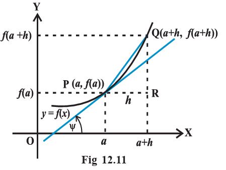
For P = (a, f(a)) and Q = (a + h, f(a + h)), the difference quotient is the slope of secant PQ. As h approaches 0, Q approaches P and the secant approaches the tangent; therefore f'(a) is the tangent's slope.
f′(a)=tanψ
Graph of y = f(x): the secant through inputs a and a + h approaches the tangent at a.
Derivative Function and Basic Derivatives
Definition
Derivative Function — Wherever the limit exists, the function f'(x) = lim as h approaches 0 of [f(x + h) - f(x)]/h is the derivative of f at x.
For 1/x, the input must satisfy x ≠ 0. The derivative of sin x at x = 0 equals 1 (with angles measured in radians).
Worked example
Find the derivative of f(x) = x².
Find the derivative function of f(x) = x² from first principles.
f′(x)=h→0limh(x+h)2−x2
Expand, cancel h, and take the limit.
=h→0limh2xh+h2=h→0lim(2x+h)=2x
Answer: f'(x) = 2x.
Power Rule
For every positive integer n, the derivative of x to the power n is n times x to the power n − 1. The result also holds for real powers, though that extension is not proved here.
dxd(xn)=nxn−1
Algebra of Derivatives
Sum, Difference, Product and Quotient Rules
For differentiable functions u and v, use these rules to differentiate sums, differences, products and quotients.