Class 11 PCM . Mathematics . Mathematics . Statistics

Chapter 13: Statistics    

Ch 13

Mathematics

Class 11 PCM

Lecture 1

Introduction & Measures Of Dispersion

Reference video · Lecture 1Introduction & Measures Of Dispersion

Central Tendency and Dispersion

Find and compare central values

  1. Add the observations and divide by their count to calculate the mean.
    xˉ=∑xin\bar{x}=\frac{\sum x_i}{n}
  2. Arrange the observations and identify the middle position or pair to calculate the median.
    n+12;n2,  n2+1\frac{n+1}{2};\quad \frac{n}{2},\;\frac{n}{2}+1
  3. Assess dispersion separately; equal mean and median do not imply equal spread.
    xˉA=xˉB,x~A=x~B⇏DA=DB\bar{x}_A=\bar{x}_B,\quad \widetilde{x}_A=\widetilde{x}_B\not\Rightarrow D_A=D_B
Worked example

Compare the last-ten-match scores of Batsmen A and B using mean, median and range.

  1. For Batsman A, the ten scores add to 530530, so the mean is 5353.
    30+91+0+64+42+80+30+5+117+7110=53010=53\frac{30+91+0+64+42+80+30+5+117+71}{10}=\frac{530}{10}=53
  2. The fifth and sixth arranged scores for A are 4242 and 6464, giving median 5353.
    42+642=53\frac{42+64}{2}=53
  3. For Batsman B, the scores also add to 530530; the fifth and sixth arranged scores are both 5353.
    53010=53;53+532=53\frac{530}{10}=53;\quad \frac{53+53}{2}=53
  4. Despite equal means and medians, their ranges differ substantially.
    RA=117−0=117;RB=60−46=14R_A=117-0=117;\quad R_B=60-46=14
Answer: Both have mean 5353 and median 5353. Batsman A's range is 117117 and Batsman B's is 1414, so A's scores are more spread out.

Range

Worked example

Find and compare the ranges of the two batsmen's scores.

  1. For Batsman A, the maximum is 117117 and the minimum is 00.
    RA=117−0=117R_A=117-0=117
  2. For Batsman B, the maximum is 6060 and the minimum is 4646.
    RB=60−46=14R_B=60-46=14
  3. A's scores have the larger range and are therefore more spread out by this measure.
    117>14117>14
Answer: Batsman A: 117117; Batsman B: 1414. A has the larger range.
⚠ Common mistake

Do not treat range as a complete description of spread: it uses only the two extreme observations and ignores the positions of all the others.

Mean Deviation

Sum of deviations from the mean

The signed deviations from the arithmetic mean always sum to zero; therefore their ordinary average is also zero.

∑i=1n(xi−xˉ)=0\sum_{i=1}^{n}(x_i-\bar{x})=0
Worked example

Find the mean deviation about the mean for 2,4,62,4,6.

  1. For the data 2,4,62,4,6, the mean is 44; their signed deviations from 44 sum to zero.
    xˉ=2+4+63=4;(2−4)+(4−4)+(6−4)=0\bar{x}=\frac{2+4+6}{3}=4;\quad (2-4)+(4-4)+(6-4)=0
  2. Take absolute values of the deviations to measure distances from the mean.
    ∣2−4∣+∣4−4∣+∣6−4∣=2+0+2=4|2-4|+|4-4|+|6-4|=2+0+2=4
  3. Divide the sum of absolute deviations by the number of observations.
    MD⁡(4)=43\operatorname{MD}(4)=\frac{4}{3}
Answer: The mean is 44, and the mean deviation about the mean is 43\frac{4}{3}.
⚠ Common mistake

Do not average signed deviations to measure dispersion: deviations from the mean sum to zero. Use absolute deviations in mean deviation.

Practice

Find the range of 3,7,9,12,153,7,9,12,15.

Hint: Subtract the smallest observation from the largest.
Key step: Identify xmax⁡=15x_{\max}=15 and xmin⁡=3x_{\min}=3.
Solution: R=15−3=12R=15-3=12.
Practice

Find the mean deviation about the mean for 1,3,5,71,3,5,7.

Hint: Find the mean, then average the absolute deviations.
Key step: The mean is 44; the absolute deviations are 3,1,1,33,1,1,3.
Solution: xˉ=4\bar{x}=4 and MD⁡(4)=3+1+1+34=2\operatorname{MD}(4)=\frac{3+1+1+3}{4}=2.

Quick recap

  • Measures of central tendency show the centre; measures of dispersion describe the spread.
  • The main dispersion measures are range, quartile deviation, mean deviation and standard deviation; quartile deviation is excluded here.
  • Range equals the maximum observation minus the minimum observation.
  • Range gives only a rough picture because it uses only the two extreme values.
  • Mean deviation about aa is 1n∑i=1n∣xi−a∣\frac{1}{n}\sum_{i=1}^{n}|x_i-a|.
  • Signed deviations from the mean sum to zero, so mean deviation uses absolute deviations.
Lecture 2

Mean Deviation For Ungrouped Data

Reference video · Lecture 2Mean Deviation For Ungrouped Data
Definition

Mean deviation — The mean deviation about a value is the average of the absolute differences between each observation and that value.

Key ideas

  • Reference value: Mean deviation can be calculated about the mean or the median; denote the chosen value by aa.
  • Absolute deviations: Use ∣xi−a∣|x_i-a| so that negative and positive deviations do not cancel.
  • Ungrouped data: Each observation is used individually, and the absolute deviations are divided by the number of observations.
  • Median: Arrange the data in ascending order first; for odd nn, the median is the observation in position n+12\frac{n+1}{2}.
Mean deviation about a value
M.D.(a)=1n∑i=1n∣xi−a∣\mathrm{M.D.}(a)=\frac{1}{n}\sum_{i=1}^{n}|x_i-a|

Use a=xˉa=\bar{x} for mean deviation about the mean, or a=Ma=M for mean deviation about the median.

Mean and median
M.D.(xˉ)=1n∑i=1n∣xi−xˉ∣,M.D.(M)=1n∑i=1n∣xi−M∣\mathrm{M.D.}(\bar{x})=\frac{1}{n}\sum_{i=1}^{n}|x_i-\bar{x}|,\qquad \mathrm{M.D.}(M)=\frac{1}{n}\sum_{i=1}^{n}|x_i-M|

The mean is xˉ\bar{x}; the median is MM.

Finding mean deviation

  1. Find the chosen centre, either the mean or the median.
    a=xˉ or a=Ma=\bar{x}\ \text{or}\ a=M
  2. Subtract the centre from each observation.
    xi−ax_i-a
  3. Take the absolute value of every deviation.
    ∣xi−a∣|x_i-a|
  4. Add the absolute deviations and divide by the number of observations.
    M.D.(a)=∑i=1n∣xi−a∣n\mathrm{M.D.}(a)=\frac{\sum_{i=1}^{n}|x_i-a|}{n}
Worked example

Find the mean deviation about the mean for 6,7,10,12,13,4,8,126,7,10,12,13,4,8,12.

  1. Find the mean of the observations 6,7,10,12,13,4,8,126,7,10,12,13,4,8,12.
    xˉ=6+7+10+12+13+4+8+128=728=9\bar{x}=\frac{6+7+10+12+13+4+8+12}{8}=\frac{72}{8}=9
  2. Find each deviation from the mean.
    xi−xˉ=−3,−2,1,3,4,−5,−1,3x_i-\bar{x}=-3,-2,1,3,4,-5,-1,3
  3. Take the absolute values and add them.
    ∣xi−xˉ∣=3,2,1,3,4,5,1,3;∑i=18∣xi−xˉ∣=22|x_i-\bar{x}|=3,2,1,3,4,5,1,3;\qquad \sum_{i=1}^{8}|x_i-\bar{x}|=22
  4. Divide the total absolute deviation by the number of observations.
    M.D.(xˉ)=228=2.75\mathrm{M.D.}(\bar{x})=\frac{22}{8}=2.75
Answer: The mean deviation about the mean is 2.752.75.
⚠ Common mistake

Do not average the signed deviations: take absolute values first, or positive and negative deviations may cancel.

Practice

Find the mean deviation about the mean for 12,3,18,17,4,9,17,19,20,15,8,17,2,3,16,11,3,1,0,512,3,18,17,4,9,17,19,20,15,8,17,2,3,16,11,3,1,0,5.

Hint: Find the mean first, then sum all absolute deviations.
Key step: xˉ=10\bar{x}=10 and ∑∣xi−xˉ∣=124\sum |x_i-\bar{x}|=124.
Solution: M.D.(xˉ)=12420=6.2\mathrm{M.D.}(\bar{x})=\frac{124}{20}=6.2.
Practice

Find the mean deviation about the median for 3,9,5,3,12,10,18,4,7,19,213,9,5,3,12,10,18,4,7,19,21.

Hint: Sort the observations and identify the sixth observation as the median.
Key step: M=9M=9 and ∑∣xi−M∣=58\sum |x_i-M|=58.
Solution: M.D.(M)=5811≈5.27\mathrm{M.D.}(M)=\frac{58}{11}\approx5.27.

Quick recap

  • Mean deviation is the average of the absolute deviations from a chosen centre.
  • Choose the mean or median as the centre before calculating.
  • Use absolute deviations so all contributions are non-negative.
  • For ungrouped data, divide the sum of absolute deviations by nn.
  • For an odd number of observations, sort the data to locate the median.
Lecture 3

Mean Deviation For Grouped Data

Reference video · Lecture 3Mean Deviation For Grouped Data

Discrete Frequency Distributions

Definition

Discrete frequency distribution — A distribution listing distinct values xix_i with their corresponding frequencies fif_i.

Key ideas

  • Total frequency: N=∑fiN=\sum f_i.
  • Weighted data: Each distinct value contributes according to its frequency.
  • Absolute deviation: Use the non-negative distance from the chosen central value.

Mean Deviation About the Mean: Discrete Data

Definition

Mean deviation about the mean — The frequency-weighted average of the absolute deviations of observations from their mean.

Mean and Mean Deviation About the Mean
xˉ=∑fixiN,M.D.(xˉ)=∑fi∣xi−xˉ∣N,N=∑fi\bar{x}=\frac{\sum f_i x_i}{N},\qquad \mathrm{M.D.}(\bar{x})=\frac{\sum f_i|x_i-\bar{x}|}{N},\qquad N=\sum f_i

Find the weighted mean first, then calculate deviations from it.

Finding Mean Deviation About the Mean

  1. Calculate the total frequency and the weighted mean.
    xˉ=∑fixiN\bar{x}=\frac{\sum f_i x_i}{N}
  2. Find each absolute deviation and multiply it by its frequency.
    fi∣xi−xˉ∣f_i|x_i-\bar{x}|
  3. Add the weighted deviations and divide by the total frequency.
    M.D.(xˉ)=∑fi∣xi−xˉ∣N\mathrm{M.D.}(\bar{x})=\frac{\sum f_i|x_i-\bar{x}|}{N}
Worked example

Find the mean deviation about the mean for the given discrete frequency distribution.

  1. For values 2,5,6,8,10,122,5,6,8,10,12 with frequencies 2,8,10,7,8,52,8,10,7,8,5, calculate the totals.
    N=40,∑fixi=300N=40,\qquad \sum f_i x_i=300
  2. Find the weighted mean.
    xˉ=30040=7.5\bar{x}=\frac{300}{40}=7.5
  3. The frequency-weighted absolute deviations sum to 9292.
    ∑fi∣xi−xˉ∣=92\sum f_i|x_i-\bar{x}|=92
  4. Divide by the total frequency to obtain the mean deviation.
    M.D.(xˉ)=9240=2.3\mathrm{M.D.}(\bar{x})=\frac{92}{40}=2.3
Answer: M.D.(xˉ)=2.3\mathrm{M.D.}(\bar{x})=2.3.

Mean Deviation About the Median: Discrete Data

Definition

Median of a discrete frequency distribution — The middle observation in the ordered data, or the average of the two middle observations when the total frequency is even.

Locating the median

  • Cumulative frequency: Add frequencies successively to locate the central observation(s).
  • Odd NN: The median is the observation at position N+12\frac{N+1}{2}.
  • Even NN: Average the observations at positions N2\frac{N}{2} and N2+1\frac{N}{2}+1.
Mean Deviation About the Median
M.D.(M)=∑fi∣xi−M∣N\mathrm{M.D.}(M)=\frac{\sum f_i|x_i-M|}{N}

Here MM denotes the median.

Finding Mean Deviation About the Median

  1. Arrange values in ascending order and calculate cumulative frequencies.
  2. Use the central observation(s) to identify the median.
    MM
  3. Calculate and sum the frequency-weighted absolute deviations, then divide by NN.
    M.D.(M)=∑fi∣xi−M∣N\mathrm{M.D.}(M)=\frac{\sum f_i|x_i-M|}{N}
Worked example

Find the mean deviation about the median for the given discrete frequency distribution.

  1. For values 3,6,9,12,13,15,21,223,6,9,12,13,15,21,22 with frequencies 3,4,5,2,4,5,4,33,4,5,2,4,5,4,3, find the total frequency and middle observations.
    N=30,x(15)=13,x(16)=13N=30,\qquad x_{(15)}=13,\qquad x_{(16)}=13
  2. Both middle observations are 1313, so the median is 1313.
    M=13+132=13M=\frac{13+13}{2}=13
  3. The weighted absolute deviations sum to 149149.
    ∑fi∣xi−M∣=149\sum f_i|x_i-M|=149
  4. Divide by the total frequency.
    M.D.(M)=14930≈4.97\mathrm{M.D.}(M)=\frac{149}{30}\approx4.97
Answer: M=13M=13 and M.D.(M)≈4.97\mathrm{M.D.}(M)\approx4.97.

Continuous Frequency Distributions

Definition

Continuous frequency distribution — A distribution that groups data into adjoining class intervals and gives the frequency in each interval.

Grouped-data representation

  • Class midpoint: Represent each interval by its midpoint xix_i in calculations.
  • Frequency: Use the class frequency fif_i as the weight for its midpoint.
  • Example: Marks intervals 00–1010, 1010–2020, 2020–3030, 3030–4040, 4040–5050, 5050–6060 can have frequencies 12,18,27,20,17,612,18,27,20,17,6.

Mean Deviation About the Mean: Continuous Data

Key procedure

  • Midpoints: Use each class midpoint xix_i as its representative observation.
  • Mean: Find the weighted average of the midpoints.
  • Mean deviation: Average the frequency-weighted absolute distances from the mean.
Grouped Mean and Mean Deviation
xˉ=∑fixiN,M.D.(xˉ)=∑fi∣xi−xˉ∣N,N=∑fi\bar{x}=\frac{\sum f_i x_i}{N},\qquad \mathrm{M.D.}(\bar{x})=\frac{\sum f_i|x_i-\bar{x}|}{N},\qquad N=\sum f_i

Use class midpoints as xix_i; the formulas are otherwise the same as for discrete data.

Using Class Midpoints

  1. Find each class midpoint, then calculate NN and the weighted sum.
    xi=lower limit+upper limit2x_i=\frac{\text{lower limit}+\text{upper limit}}{2}
  2. Calculate the weighted mean.
    xˉ=∑fixiN\bar{x}=\frac{\sum f_i x_i}{N}
  3. Weight each absolute deviation by its frequency, then divide the total by NN.
    M.D.(xˉ)=∑fi∣xi−xˉ∣N\mathrm{M.D.}(\bar{x})=\frac{\sum f_i|x_i-\bar{x}|}{N}
Worked example

Find the mean deviation about the mean for the grouped marks data.

  1. For classes 1010–2020, 2020–3030, 3030–4040, 4040–5050, 5050–6060, 6060–7070, 7070–8080 with frequencies 2,3,8,14,8,3,22,3,8,14,8,3,2, calculate the midpoints and totals.
    xi=15,25,35,45,55,65,75,N=40,∑fixi=1800x_i=15,25,35,45,55,65,75,\qquad N=40,\qquad \sum f_i x_i=1800
  2. Find the mean.
    xˉ=180040=45\bar{x}=\frac{1800}{40}=45
  3. The weighted absolute deviations from the mean sum to 400400.
    ∑fi∣xi−xˉ∣=400\sum f_i|x_i-\bar{x}|=400
  4. Divide by the total frequency.
    M.D.(xˉ)=40040=10\mathrm{M.D.}(\bar{x})=\frac{400}{40}=10
Answer: M.D.(xˉ)=10\mathrm{M.D.}(\bar{x})=10.

Shortcut: Step-Deviation Method

Definition

Step deviation — A scaled deviation from an assumed mean, used to simplify calculations of the grouped mean.

Key ideas

  • Assumed mean: Choose a convenient value aa, usually near the centre of the data.
  • Scale factor: Choose a common factor hh of the deviations, when available.
  • Step deviations: Set di=xi−ahd_i=\frac{x_i-a}{h}; this shifts and rescales the values.
  • Use: Step deviation simplifies finding the mean; calculate mean deviation using the original midpoints.
Mean by Step Deviation
di=xi−ah,xˉ=a+h∑fidiNd_i=\frac{x_i-a}{h},\qquad \bar{x}=a+h\frac{\sum f_i d_i}{N}

After finding the mean this way, use the usual formula for mean deviation.

Worked example

Find the mean and mean deviation for the grouped data by step deviation.

  1. For the previous grouped data, choose the assumed mean a=45a=45 and scale factor h=10h=10.
    di=xi−4510d_i=\frac{x_i-45}{10}
  2. The step deviations are −3,−2,−1,0,1,2,3-3,-2,-1,0,1,2,3; their weighted sum is zero.
    ∑fidi=0\sum f_i d_i=0
  3. Apply the step-deviation formula to find the mean.
    xˉ=45+10(040)=45\bar{x}=45+10\left(\frac{0}{40}\right)=45
  4. Use the original midpoints to calculate mean deviation; the weighted distances total 400400.
    M.D.(xˉ)=40040=10\mathrm{M.D.}(\bar{x})=\frac{400}{40}=10
Answer: xˉ=45\bar{x}=45 and M.D.(xˉ)=10\mathrm{M.D.}(\bar{x})=10.

Mean Deviation About the Median: Continuous Data

Definition

Median class — The class interval whose cumulative frequency first reaches or exceeds half the total frequency.

Grouped Median and Mean Deviation
M=l+N2−Cfh,M.D.(M)=∑fi∣xi−M∣NM=l+\frac{\frac{N}{2}-C}{f}h,\qquad \mathrm{M.D.}(M)=\frac{\sum f_i|x_i-M|}{N}

Here ll is the median-class lower limit, CC the cumulative frequency before it, ff its frequency, and hh its width.

Finding Mean Deviation About the Grouped Median

  1. Calculate cumulative frequencies and identify the median class containing the N2\frac{N}{2}th observation.
  2. Apply the grouped median formula.
    M=l+N2−CfhM=l+\frac{\frac{N}{2}-C}{f}h
  3. Find each midpoint's absolute deviation from the median, weight by frequency, and divide the sum by NN.
    M.D.(M)=∑fi∣xi−M∣N\mathrm{M.D.}(M)=\frac{\sum f_i|x_i-M|}{N}
Worked example

Find the mean deviation about the median for the grouped data.

  1. For classes 00–1010, 1010–2020, 2020–3030, 3030–4040, 4040–5050, 5050–6060 with frequencies 6,7,15,16,4,26,7,15,16,4,2, the total frequency is 5050.
    N=50,N2=25N=50,\qquad \frac{N}{2}=25
  2. The 2525th observation falls in the class 2020–3030; thus l=20l=20, C=13C=13, f=15f=15, and h=10h=10.
    M=20+25−1315×10=28M=20+\frac{25-13}{15}\times10=28
  3. Using midpoints 5,15,25,35,45,555,15,25,35,45,55, the weighted absolute deviations sum to 508508.
    ∑fi∣xi−M∣=508\sum f_i|x_i-M|=508
  4. Divide by the total frequency.
    M.D.(M)=50850=10.16\mathrm{M.D.}(M)=\frac{508}{50}=10.16
Answer: M=28M=28 and M.D.(M)=10.16\mathrm{M.D.}(M)=10.16.

Limitations of Mean Deviation

Limitations

  • Unrepresentative median: With very high variability, the median may not represent the series well, making mean deviation about it unreliable.
  • About the mean: The sum of absolute deviations about the mean is generally not smaller than that about the median, so mean deviation about the mean may be unsatisfactory.
  • Absolute values: Using absolute deviations prevents mean deviation from being treated easily by further algebraic methods.
  • Alternative: Standard deviation is another measure of dispersion.
Practice

For values 1,3,51,3,5 with frequencies 2,3,12,3,1, find the mean deviation about the mean.

Hint: Find the weighted mean before taking absolute deviations.
Key step: N=6N=6, xˉ=166=83\bar{x}=\frac{16}{6}=\frac{8}{3}, and ∑fi∣xi−xˉ∣=203\sum f_i|x_i-\bar{x}|=\frac{20}{3}.
Solution: M.D.(xˉ)=20/36=109\mathrm{M.D.}(\bar{x})=\frac{20/3}{6}=\frac{10}{9}.
Practice

For classes 00–1010, 1010–2020, 2020–3030 with frequencies 2,5,32,5,3, find the mean deviation about the mean.

Hint: Use midpoints 5,15,255,15,25.
Key step: N=10N=10, xˉ=16\bar{x}=16, and ∑fi∣xi−16∣=54\sum f_i|x_i-16|=54.
Solution: M.D.(xˉ)=5410=5.4\mathrm{M.D.}(\bar{x})=\frac{54}{10}=5.4.
Practice

For classes 00–1010, 1010–2020, 2020–3030 with frequencies 2,5,32,5,3, find the mean deviation about the median.

Hint: The median class is 1010–2020; use the grouped median formula.
Key step: M=10+5−25×10=16M=10+\frac{5-2}{5}\times10=16, and ∑fi∣xi−M∣=54\sum f_i|x_i-M|=54.
Solution: M.D.(M)=5410=5.4\mathrm{M.D.}(M)=\frac{54}{10}=5.4.

Quick recap

  • For discrete data, use distinct values xix_i and frequencies fif_i; for continuous data, use class midpoints.
  • Mean deviation about the mean is ∑fi∣xi−xˉ∣N\frac{\sum f_i|x_i-\bar{x}|}{N}.
  • For discrete data, cumulative frequencies locate the middle observation(s) used to find the median.
  • For continuous data, use M=l+N2−CfhM=l+\frac{\frac{N}{2}-C}{f}h to find the grouped median.
  • Mean deviation about the median is ∑fi∣xi−M∣N\frac{\sum f_i|x_i-M|}{N}.
  • Step deviation simplifies calculating the mean; use original midpoints for mean-deviation distances.
  • Absolute values limit further algebraic treatment of mean deviation; standard deviation is an alternative.
Lecture 4

Variance And Standard Deviation

Reference video · Lecture 4Variance And Standard Deviation

Squared Deviations and Variance

Definition

Variance — Variance is the mean of the squared deviations of observations from their arithmetic mean; it measures their dispersion.

Properties of squared deviations

Squaring deviations makes them non-negative, so positive and negative deviations cannot cancel. The sum of squared deviations alone depends on the number of observations; averaging the squares gives a more suitable comparison of dispersion. Variance is zero exactly when all observations equal the mean.

Why use the mean of squared deviations?
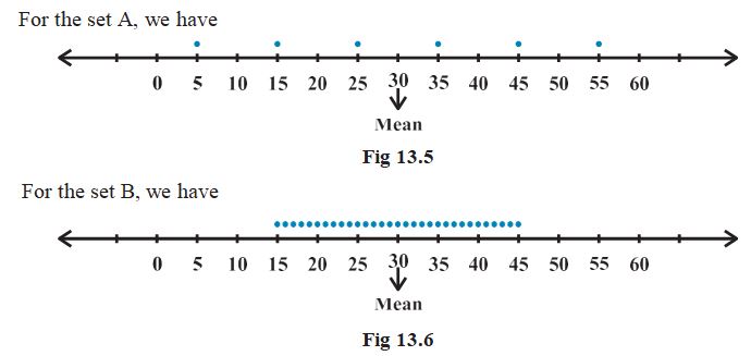
Data setNumber of observationsMeanSum of squared deviationsMean of squared deviations
A: 5,15,25,35,45,555,15,25,35,45,55663030175017501750/6≈291.671750/6\approx291.67
B: integers from 1515 to 454531313030248024802480/31=802480/31=80
Sum of the first n squares
∑k=1nk2=n(n+1)(2n+1)6\sum_{k=1}^{n}k^2=\frac{n(n+1)(2n+1)}{6}

Useful for calculating the sum of squared deviations in set B.

Comparing the sets

  • Set B: Its squared-deviation total is 2∑k=115k2=2(15⋅16⋅316)=24802\sum_{k=1}^{15}k^2=2\left(\frac{15\cdot16\cdot31}{6}\right)=2480.
  • Conclusion: Set A has the greater dispersion: its mean squared deviation is about 291.67291.67, compared with 8080 for set B.
Dot plots compare sets A and B on number lines; both have mean 30.
Dot plots compare sets A and B on number lines; both have mean 3030.
Variance of ungrouped data
σ2=1n∑i=1n(xi−xˉ)2\sigma^2=\frac{1}{n}\sum_{i=1}^{n}(x_i-\bar{x})^2

Use when all nn observations are listed individually.

Calculate variance from ungrouped data

  1. Find the mean of the observations.
    xˉ=∑i=1nxin\bar{x}=\frac{\sum_{i=1}^{n}x_i}{n}
  2. Calculate each deviation from the mean and square it.
    (xi−xˉ)2(x_i-\bar{x})^2
  3. Add the squared deviations and divide by the number of observations.
    σ2=∑i=1n(xi−xˉ)2n\sigma^2=\frac{\sum_{i=1}^{n}(x_i-\bar{x})^2}{n}

Standard Deviation

Definition

Standard deviation — Standard deviation is the positive square root of variance and is a measure of dispersion expressed in the original units of the data.

Relationship between variance and standard deviation

Variance is measured in squared data units, while standard deviation has the same units as the observations.

σ=σ2=1n∑i=1n(xi−xˉ)2\sigma=\sqrt{\sigma^2}=\sqrt{\frac{1}{n}\sum_{i=1}^{n}(x_i-\bar{x})^2}
Worked example

Find the variance and standard deviation of 6,8,10,12,14,16,18,20,22,246,8,10,12,14,16,18,20,22,24.

  1. Find the variance and standard deviation of 6,8,10,12,14,16,18,20,22,246,8,10,12,14,16,18,20,22,24.
  2. Find the mean.
    xˉ=6+8+10+12+14+16+18+20+22+2410=15\bar{x}=\frac{6+8+10+12+14+16+18+20+22+24}{10}=15
  3. Calculate and add the squared deviations from the mean.
    ∑i=110(xi−15)2=81+49+25+9+1+1+9+25+49+81=330\sum_{i=1}^{10}(x_i-15)^2=81+49+25+9+1+1+9+25+49+81=330
  4. Divide by the number of observations to find variance.
    σ2=33010=33\sigma^2=\frac{330}{10}=33
  5. Take the positive square root to find standard deviation.
    σ=33≈5.74\sigma=\sqrt{33}\approx5.74
Answer: σ2=33\sigma^2=33 and σ=33≈5.74\sigma=\sqrt{33}\approx5.74.

Discrete Frequency Distributions

Definition

Discrete frequency distribution — A discrete frequency distribution lists each distinct value xix_i together with its frequency fif_i.

Frequency-weighted dispersion

Each squared deviation contributes once for every occurrence of its value. The total number of observations is N=∑i=1nfiN=\sum_{i=1}^{n}f_i.

xˉ=∑i=1nfixiN,σ2=1N∑i=1nfi(xi−xˉ)2,σ=σ2\bar{x}=\frac{\sum_{i=1}^{n}f_ix_i}{N},\qquad \sigma^2=\frac{1}{N}\sum_{i=1}^{n}f_i(x_i-\bar{x})^2,\qquad \sigma=\sqrt{\sigma^2}

Calculate variance from a discrete frequency distribution

  1. Find the total frequency and the weighted mean.
    N=∑fi,xˉ=∑fixiNN=\sum f_i,\qquad \bar{x}=\frac{\sum f_ix_i}{N}
  2. For each value, find its squared deviation and multiply by its frequency.
    fi(xi−xˉ)2f_i(x_i-\bar{x})^2
  3. Add the weighted squared deviations and divide by the total frequency; then take the positive square root for standard deviation.
    σ2=∑fi(xi−xˉ)2N,σ=σ2\sigma^2=\frac{\sum f_i(x_i-\bar{x})^2}{N},\qquad \sigma=\sqrt{\sigma^2}
Practice

For the observations 2,4,62,4,6, find the variance and standard deviation.

Hint: First find the mean, then use the squared deviations.
Key step: xˉ=4\bar{x}=4 and ∑(xi−xˉ)2=8\sum(x_i-\bar{x})^2=8.
Solution: σ2=83\sigma^2=\frac{8}{3} and σ=83≈1.63\sigma=\sqrt{\frac{8}{3}}\approx1.63.
Practice

For xi:4,8,11,17,20,24,32x_i:4,8,11,17,20,24,32 and fi:3,5,9,5,4,3,1f_i:3,5,9,5,4,3,1, find the variance and standard deviation.

Hint: Compute NN and the weighted mean first, then total the frequency-weighted squared deviations.
Key step: N=30N=30, xˉ=14\bar{x}=14, and ∑fi(xi−xˉ)2=1374\sum f_i(x_i-\bar{x})^2=1374.
Solution: σ2=137430=45.8\sigma^2=\frac{1374}{30}=45.8 and σ=45.8≈6.77\sigma=\sqrt{45.8}\approx6.77.
⚠ Common mistake

Do not divide by nn or NN before finding the sum of squared deviations; for a frequency distribution, include each value's frequency in both the weighted mean and the variance calculation.

Quick recap

  • Squaring deviations prevents positive and negative deviations from cancelling.
  • The sum of squared deviations depends on the number of observations; variance averages those squares.
  • For ungrouped data, σ2=1n∑(xi−xˉ)2\sigma^2=\frac{1}{n}\sum(x_i-\bar{x})^2.
  • Use ∑k=1nk2=n(n+1)(2n+1)6\sum_{k=1}^{n}k^2=\frac{n(n+1)(2n+1)}{6} to calculate sums of consecutive squares.
  • Standard deviation is the positive square root of variance and uses the original data units.
  • For a discrete frequency distribution, use N=∑fiN=\sum f_i and weight each squared deviation by fif_i; variance is zero only when every observation equals the mean.
Lecture 5

Standard Deviation Of A Continuous Frequency Distribution

Reference video · Lecture 5Standard Deviation Of A Continuous Frequency Distribution

Midpoints and the Direct Method

Variance and standard deviation

For grouped data, variance is the frequency-weighted mean of squared deviations from the mean; standard deviation is its positive square root.

σ2=1N∑i=1nfi(xi−xˉ)2,σ=1N∑i=1nfi(xi−xˉ)2\sigma^2=\frac{1}{N}\sum_{i=1}^{n}f_i(x_i-\bar{x})^2,\qquad \sigma=\sqrt{\frac{1}{N}\sum_{i=1}^{n}f_i(x_i-\bar{x})^2}
Equivalent formula using sums
σ2=∑fixi2N−(∑fixiN)2=N∑fixi2−(∑fixi)2N2,σ=1NN∑fixi2−(∑fixi)2\sigma^2=\frac{\sum f_i x_i^2}{N}-\left(\frac{\sum f_i x_i}{N}\right)^2=\frac{N\sum f_i x_i^2-(\sum f_i x_i)^2}{N^2},\qquad \sigma=\frac{1}{N}\sqrt{N\sum f_i x_i^2-(\sum f_i x_i)^2}

Use this form when the totals ∑fixi\sum f_i x_i and ∑fixi2\sum f_i x_i^2 are easier to calculate.

Direct method

  1. Find every class midpoint and calculate the total frequency.
    xi=ai+bi2,N=∑fix_i=\frac{a_i+b_i}{2},\qquad N=\sum f_i
  2. Calculate the mean of the distribution.
    xˉ=∑fixiN\bar{x}=\frac{\sum f_i x_i}{N}
  3. Find the weighted sum of squared deviations, then calculate variance and standard deviation.
    σ2=∑fi(xi−xˉ)2N,σ=σ2\sigma^2=\frac{\sum f_i(x_i-\bar{x})^2}{N},\qquad \sigma=\sqrt{\sigma^2}
Worked example

Find the mean, variance and standard deviation of the given continuous frequency distribution.

  1. For classes 3030–4040 through 9090–100100 with frequencies 3,7,12,15,8,3,23,7,12,15,8,3,2, the midpoints are 35,45,55,65,75,85,9535,45,55,65,75,85,95.
    N=50,∑fixi=3100N=50,\qquad \sum f_i x_i=3100
  2. Calculate the mean.
    xˉ=310050=62\bar{x}=\frac{3100}{50}=62
  3. The weighted sum of squared deviations is 1005010050.
    ∑fi(xi−62)2=10050\sum f_i(x_i-62)^2=10050
  4. Calculate variance and standard deviation.
    σ2=1005050=201,σ=201≈14.18\sigma^2=\frac{10050}{50}=201,\qquad \sigma=\sqrt{201}\approx14.18
Answer: xˉ=62\bar{x}=62, σ2=201\sigma^2=201, and σ≈14.18\sigma\approx14.18.

Discrete-data check for the equivalent formula

  • Data: For xi=3,8,13,18,23x_i=3,8,13,18,23 and fi=7,10,15,10,6f_i=7,10,15,10,6, the totals are N=48N=48, ∑fixi=614\sum f_i x_i=614, and ∑fixi2=9652\sum f_i x_i^2=9652.
  • Calculation: σ=14848(9652)−6142=293.7748≈6.12\sigma=\frac{1}{48}\sqrt{48(9652)-614^2}=\frac{293.77}{48}\approx6.12.
  • Result: The standard deviation is approximately 6.126.12.

Shortcut (Step-Deviation) Method

Shortcut formulas
xˉ=A+h∑fiyiN,σ2=h2N2[N∑fiyi2−(∑fiyi)2],σ=hNN∑fiyi2−(∑fiyi)2\bar{x}=A+h\frac{\sum f_i y_i}{N},\qquad \sigma^2=\frac{h^2}{N^2}\left[N\sum f_i y_i^2-(\sum f_i y_i)^2\right],\qquad \sigma=\frac{h}{N}\sqrt{N\sum f_i y_i^2-(\sum f_i y_i)^2}

Use coded values yiy_i and their frequencies to calculate the mean, variance and standard deviation.

Step-deviation procedure

  1. Choose an assumed mean AA and class width hh; calculate the coded value for each midpoint.
    yi=xi−Ahy_i=\frac{x_i-A}{h}
  2. Calculate the required frequency totals.
    N=∑fi,∑fiyi,∑fiyi2N=\sum f_i,\qquad \sum f_i y_i,\qquad \sum f_i y_i^2
  3. Substitute the totals into the shortcut formulas.
    xˉ=A+h∑fiyiN,σ2=h2N2[N∑fiyi2−(∑fiyi)2]\bar{x}=A+h\frac{\sum f_i y_i}{N},\qquad \sigma^2=\frac{h^2}{N^2}\left[N\sum f_i y_i^2-(\sum f_i y_i)^2\right]
  4. Take the positive square root of the variance to obtain standard deviation.
    σ=σ2\sigma=\sqrt{\sigma^2}

Shortcut calculation for the grouped distribution

  • Coding: For the same classes, choose A=65A=65 and h=10h=10; the coded values are −3,−2,−1,0,1,2,3-3,-2,-1,0,1,2,3.
  • Totals: N=50N=50, ∑fiyi=−15\sum f_i y_i=-15, and ∑fiyi2=105\sum f_i y_i^2=105.
  • Mean: xˉ=65+10(−1550)=62\bar{x}=65+10\left(\frac{-15}{50}\right)=62.
  • Variance and standard deviation: σ2=102502[50(105)−(−15)2]=201\sigma^2=\frac{10^2}{50^2}[50(105)-(-15)^2]=201, so σ=201≈14.18\sigma=\sqrt{201}\approx14.18.

Effect of Changing Observations

Translation and scaling properties

Adding a constant to every observation leaves variance unchanged; multiplying every observation by kk multiplies variance by k2k^2 and standard deviation by ∣k∣|k|.

Var⁡(xi+a)=Var⁡(xi),Var⁡(kxi)=k2Var⁡(xi)\operatorname{Var}(x_i+a)=\operatorname{Var}(x_i),\qquad \operatorname{Var}(kx_i)=k^2\operatorname{Var}(x_i)
⚠ Common mistake

Do not multiply standard deviation by k2k^2: multiplying observations by kk multiplies standard deviation by ∣k∣|k|, while variance is multiplied by k2k^2.

Practice

A data set has variance 55. Find the variance and standard deviation after every observation is multiplied by 22.

Hint: Use the scaling rule for variance and standard deviation.
Key step: σy2=22σx2\sigma_y^2=2^2\sigma_x^2.
Solution: New variance =4(5)=20=4(5)=20; new standard deviation =20=25≈4.47=\sqrt{20}=2\sqrt{5}\approx4.47.
Practice

The mean of five observations is 4.44.4, and their variance is 8.248.24. Three observations are 1,2,61,2,6. Find the other two observations.

Hint: Use the mean to find x+yx+y, then use the variance to find x2+y2x^2+y^2.
Key step: x+y=13x+y=13 and x2+y2=97x^2+y^2=97, so (x−y)2=25(x-y)^2=25.
Solution: From the mean, x+y=22−9=13x+y=22-9=13. From the variance, ∑(xi−4.4)2=5(8.24)=41.2\sum (x_i-4.4)^2=5(8.24)=41.2, giving x2+y2=97x^2+y^2=97. Then 2xy=132−97=722xy=13^2-97=72, so (x−y)2=97−72=25(x-y)^2=97-72=25. Thus the remaining observations are 44 and 99.
Practice

For 100100 observations, an incorrect mean of 4040 and standard deviation of 5.15.1 were obtained because 5050 was recorded instead of 4040. Find the correct mean and standard deviation.

Hint: Correct both ∑xi\sum x_i and ∑xi2\sum x_i^2 before recalculating.
Key step: ∑xi=4000−50+40=3990\sum x_i=4000-50+40=3990; correct ∑xi2=162601−502+402=161701\sum x_i^2=162601-50^2+40^2=161701.
Solution: Correct mean =3990/100=39.9=3990/100=39.9. The incorrect sum of squares is 100(5.12+402)=162601100(5.1^2+40^2)=162601. Hence the corrected sum of squares is 162601−2500+1600=161701162601-2500+1600=161701. Correct variance =161701/100−(39.9)2=25=161701/100-(39.9)^2=25, so the correct standard deviation is 55.

Quick recap

  • Represent every continuous class by its midpoint and retain its frequency.
  • Compute N=∑fiN=\sum f_i and xˉ=∑fixiN\bar{x}=\frac{\sum f_i x_i}{N}.
  • Use σ2=∑fi(xi−xˉ)2N\sigma^2=\frac{\sum f_i(x_i-\bar{x})^2}{N} and σ=σ2\sigma=\sqrt{\sigma^2}.
  • The equivalent raw-sum formula uses ∑fixi\sum f_i x_i and ∑fixi2\sum f_i x_i^2.
  • Step-deviation uses yi=xi−Ahy_i=\frac{x_i-A}{h} to simplify calculations; then xˉ=A+h∑fiyiN\bar{x}=A+h\frac{\sum f_i y_i}{N}.
  • Adding a constant does not change variance; scaling observations by kk scales variance by k2k^2 and standard deviation by ∣k∣|k|.

Formula sheet

Mean deviation about a value
M.D.(a)=1n∑i=1n∣xi−a∣\mathrm{M.D.}(a)=\frac{1}{n}\sum_{i=1}^{n}|x_i-a|
Mean and median
M.D.(xˉ)=1n∑i=1n∣xi−xˉ∣,M.D.(M)=1n∑i=1n∣xi−M∣\mathrm{M.D.}(\bar{x})=\frac{1}{n}\sum_{i=1}^{n}|x_i-\bar{x}|,\qquad \mathrm{M.D.}(M)=\frac{1}{n}\sum_{i=1}^{n}|x_i-M|
Mean and Mean Deviation About the Mean
xˉ=∑fixiN,M.D.(xˉ)=∑fi∣xi−xˉ∣N,N=∑fi\bar{x}=\frac{\sum f_i x_i}{N},\qquad \mathrm{M.D.}(\bar{x})=\frac{\sum f_i|x_i-\bar{x}|}{N},\qquad N=\sum f_i
Mean Deviation About the Median
M.D.(M)=∑fi∣xi−M∣N\mathrm{M.D.}(M)=\frac{\sum f_i|x_i-M|}{N}
Grouped Mean and Mean Deviation
xˉ=∑fixiN,M.D.(xˉ)=∑fi∣xi−xˉ∣N,N=∑fi\bar{x}=\frac{\sum f_i x_i}{N},\qquad \mathrm{M.D.}(\bar{x})=\frac{\sum f_i|x_i-\bar{x}|}{N},\qquad N=\sum f_i
Mean by Step Deviation
di=xi−ah,xˉ=a+h∑fidiNd_i=\frac{x_i-a}{h},\qquad \bar{x}=a+h\frac{\sum f_i d_i}{N}
Grouped Median and Mean Deviation
M=l+N2−Cfh,M.D.(M)=∑fi∣xi−M∣NM=l+\frac{\frac{N}{2}-C}{f}h,\qquad \mathrm{M.D.}(M)=\frac{\sum f_i|x_i-M|}{N}
Sum of the first n squares
∑k=1nk2=n(n+1)(2n+1)6\sum_{k=1}^{n}k^2=\frac{n(n+1)(2n+1)}{6}
Variance of ungrouped data
σ2=1n∑i=1n(xi−xˉ)2\sigma^2=\frac{1}{n}\sum_{i=1}^{n}(x_i-\bar{x})^2
Equivalent formula using sums
σ2=∑fixi2N−(∑fixiN)2=N∑fixi2−(∑fixi)2N2,σ=1NN∑fixi2−(∑fixi)2\sigma^2=\frac{\sum f_i x_i^2}{N}-\left(\frac{\sum f_i x_i}{N}\right)^2=\frac{N\sum f_i x_i^2-(\sum f_i x_i)^2}{N^2},\qquad \sigma=\frac{1}{N}\sqrt{N\sum f_i x_i^2-(\sum f_i x_i)^2}
Shortcut formulas
xˉ=A+h∑fiyiN,σ2=h2N2[N∑fiyi2−(∑fiyi)2],σ=hNN∑fiyi2−(∑fiyi)2\bar{x}=A+h\frac{\sum f_i y_i}{N},\qquad \sigma^2=\frac{h^2}{N^2}\left[N\sum f_i y_i^2-(\sum f_i y_i)^2\right],\qquad \sigma=\frac{h}{N}\sqrt{N\sum f_i y_i^2-(\sum f_i y_i)^2}

Mathematics — ALL CHAPTERS

1

Sets

View

2

Relations And Functions

View

3

Trigonometric Functions

View

4

Complex Numbers And Quadratic Equations

View

5

Linear  Inequalities

View

6

Permutations And Combinations

View

7

Binomial Theorem

View

8

Sequences And Series

View

9

Straight Lines

View

10

Conic Sections

View

11

Introduction To Three Dimensional Geometry

View

12

Limits And Derivatives

View

13

Statistics    

View

14

Probability

View