Class 12 PCM . Mathematics . Mathematics Part II . Linear Programming
Chapter 12: Linear Programming
Ch 12
Mathematics
Class 12 PCM
Introduction
Optimisation and Linear Programming
Optimisation problem — A problem that seeks to maximise or minimise a quantity, such as profit, cost or resource use.
Linear programming problem (LPP) — A special type of optimisation problem that finds the maximum or minimum value of a linear function subject to linear constraints and non-negativity conditions.
Key terms
- Decision variables: Unknown quantities chosen in a problem, such as the numbers of products to make or buy.
- Objective function: The linear function whose maximum or minimum is required.
- Constraints: Linear equations, inequalities or other restrictions that the decision variables must satisfy.
- Non-negative restrictions: Conditions such as and , which prevent negative quantities.
- Feasible choice: Values of the decision variables that satisfy every constraint, including non-negativity.
For two decision variables, the linear objective function has this form, where and are constants.
Furniture dealer: the optimisation situation
- Decision: The dealer chooses how many tables and chairs to buy, aiming to maximise total profit.
- Limits: The investment is at most Rs. 50,000 and storage is at most 60 items.
- Tables only: The budget allows 20 tables, yielding a profit of Rs. 5,000.
- Chairs only: Although the budget allows 100 chairs, storage limits the purchase to 60, yielding Rs. 4,500.
- Mixed purchase: 10 tables and 50 chairs use the full budget and storage capacity, yielding Rs. 6,250; this is a feasible choice, not necessarily the maximum.
Formulating an LPP
Translate a situation into a mathematical model
- Define decision variables for the quantities being chosen.
- Write the quantity to be maximised or minimised as a linear objective function.
- Translate each resource limit or requirement into a linear constraint.
- Add non-negativity conditions for the decision variables.
Formulate the furniture dealer's problem as an LPP. Also calculate the profit for 10 tables and 50 chairs.
- Let be the number of tables and the number of chairs.
- The investment cannot exceed Rs. 50,000; divide the budget inequality by 500.
- The dealer can store at most 60 items.
- The quantities bought must be non-negative.
- Profit is Rs. 250 per table and Rs. 75 per chair, so this is the objective function.
- For 10 tables and 50 chairs, both limits are met and the profit is Rs. 6,250.
Solving LPPs in this chapter
- Method covered: This chapter studies the graphical method for solving linear programming problems.
Do not confuse the objective function with the constraints: the objective is what must be maximised or minimised, while the constraints limit the choices.
A workshop makes products A and B. Each A uses 2 hours and each B uses 1 hour, with at most 40 hours available. Profit per unit is Rs. 30 for A and Rs. 20 for B. Formulate the LPP.
A farmer plants wheat and maize. Wheat earns Rs. 400 per plot and maize Rs. 300 per plot. There are at most 12 plots; wheat needs 2 units of fertiliser per plot and maize needs 1, with at most 18 units available. Formulate the LPP.
Quick recap
- An LPP is a special type of optimisation problem involving a linear objective function and linear constraints.
- Decision variables represent the quantities being chosen; constraints describe limits and requirements.
- Include non-negativity conditions such as and .
- A feasible choice satisfies all constraints, but it is not automatically optimal.
- The furniture dealer's objective is , subject to investment and storage limits.
- This chapter solves LPPs using the graphical method.
Graphical Method Of Solving Linear Programming Problems
Feasible Region and Feasible Solutions
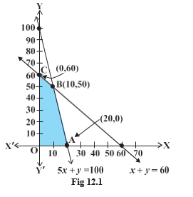
Optimal Solutions and Corner-Point Theorems
If an objective function has an optimal value on the feasible region, that value occurs at a corner point (vertex) of the region. The feasible region is a convex polygon.
If the feasible region is bounded, the objective function has both a maximum and a minimum, and each occurs at a corner point.
If the Feasible Region Is Unbounded
- Existence A maximum or minimum may not exist. If an optimum exists, it occurs at a corner point.
- Maximum test Let be the largest objective value among the corner points. It is the maximum if the open half-plane has no point in common with the feasible region.
- Minimum test Let be the smallest objective value among the corner points. It is the minimum if the open half-plane has no point in common with the feasible region.
Corner-Point Method
Steps to Solve Graphically
- Graph the constraints and identify their common feasible region.
- Find every corner point by inspection or by solving the equations of intersecting boundary lines.
- Evaluate the objective function at each corner point; note the largest value and smallest value .
- For a bounded region, and are the maximum and minimum. For an unbounded region, apply the relevant open-half-plane test.
Evaluate the objective function at every vertex of the feasible region.
Find the maximum return and the investment choice that gives it.
- Maximise the investment return; the feasible-region vertices are , , and .
- Find the intersection of the two constraint boundaries.
- Evaluate the objective function at each vertex.
| Vertex | Objective value |
|---|---|
| (maximum) | |
Maximise subject to , , and .
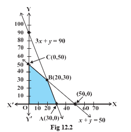
For , , and , classify , , and as feasible or infeasible.
Do not test only the constraint intercepts: include every feasible intersection of boundary lines, then compare the objective values at all vertices.
Quick recap
- The feasible region is the common set satisfying all constraints, including non-negativity.
- Points inside or on the boundary are feasible; points outside are infeasible.
- A corner point is an intersection of boundary lines.
- If an optimum exists, it occurs at a corner point.
- For a bounded region, both maximum and minimum values exist and occur at vertices.
- For an unbounded region, an optimum may not exist; check the relevant open half-plane.
- The corner-point method compares the objective values at every feasible vertex.
Graphical Method Of Solving Linear Programming Problems(Contiune)
Bounded Feasible Region: Minimum at a Corner Point
Corner-point method — For a linear programming problem with a bounded feasible region, evaluate the objective function at every vertex to find its maximum or minimum.
Find the optimum in a bounded region
- Graph the constraints and identify the feasible region and its vertices.
- Evaluate the objective function at every vertex.
- Choose the least or greatest value, as required.
Minimise subject to , , , and .
- The feasible region has vertices , and . Evaluate at each.
- Evaluate the objective at the second vertex.
- Evaluate the objective at the third vertex and compare the values.
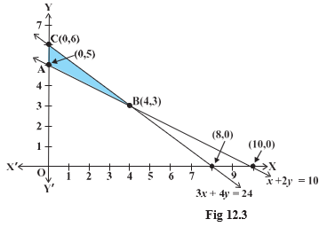
Multiple Optimal Solutions
If two vertices of the feasible region give the same optimal value, every point on the line segment joining them also gives that value.
Find the minimum and maximum of subject to , , , , and .
- The vertices are , , and . Compute at each vertex.
- The least value is at . The two vertices giving the greatest value both lie on .
- Thus all points on the segment from to have the same greatest value.
Unbounded Feasible Region
A best value at a vertex does not by itself prove an optimum when the feasible region is unbounded. For a proposed minimum , test whether the feasible region intersects the half-plane where ; for a proposed maximum , test whether it intersects the half-plane where .
Determine whether has a minimum or maximum under , , , , and .
- The feasible region is unbounded. At its listed vertices, takes the following values.
- The smallest vertex value is . To check whether it is a true minimum, test the points where .
- This strict half-plane intersects the feasible region, so feasible points have objective values below .
- For the maximum candidate , the test region does not intersect the feasible region; the maximum is attained at .
In an unbounded feasible region, do not assume the smallest or greatest vertex value is the optimum; check whether better objective values occur elsewhere in the region.
Infeasible Linear Programming Problem
Infeasible problem — A linear programming problem is infeasible if no point satisfies all its constraints simultaneously.
Check whether the constraints , , , and have a feasible solution.
- The non-negativity conditions and imply a lower bound on .
- This contradicts the constraint , so the feasible region is empty.
General Properties of Linear Programming
- Feasible region: It is always convex; the line segment between any two of its points lies entirely within it.
- Optimal value: When a finite optimum exists, it occurs at a vertex of the feasible region.
- Multiple optima: If two vertices give the same optimal value, the entire segment between them gives that value.
- Variables: The decision variables are subject to non-negativity constraints such as and .
Maximise subject to , , , , and .
Determine whether , , and are feasible.
Quick recap
- For a bounded feasible region, evaluate the objective at every vertex to find the optimum.
- Equal optimal values at two vertices mean every point between them is optimal.
- In an unbounded region, test whether points with a better objective value intersect the feasible region.
- A problem is infeasible when its constraints cannot all hold at the same time.
- The feasible region is convex, and a finite optimum occurs at a vertex.
Formula sheet
Mathematics — ALL CHAPTERS
1
Relations And Functions
2
Inverse Trigonometric Functions
3
Matrices
4
DETERMINANTS
5
Continuity And Differentiability
6
Application Of Derivatives
7
Integrals
8
APPLICATION OF INTEGRALS
9
DIFFERENTIAL EQUATIONS
10
VECTOR ALGEBRA
11
Three Dimensional Geometry
12
Linear Programming
13
Probability
14
Proofs In Mathematics
15
Mathematical Modelling