Class 12 PCM . Mathematics . Mathematics Part II . Probability
Chapter 13: Probability
Ch 13
Mathematics
Class 12 PCM
Introduction
Chapter focus and assumptions
What this chapter develops
- Starting point: Probability measures uncertainty in the outcomes of a random experiment.
- This lecture: Introduces conditional probability—probability calculated when another event is known to have occurred.
- Later ideas: Conditional probability supports Bayes’ theorem, the multiplication rule, and independence; the chapter also covers random variables, probability distributions, mean, variance, and the binomial distribution.
- Default assumption: Outcomes are treated as equally likely unless stated otherwise.
Conditional probability
Conditional probability — The conditional probability of event given that event has occurred is the probability of calculated within the restricted sample space .
For events and in the same sample space, the outcomes counted in the restricted space that also satisfy are exactly those in . The formula requires .
Key points
- Restricted space: Once is known to have occurred, outcomes outside are excluded.
- Favourable outcomes: The outcomes in that also make occur form .
- Equally likely outcomes: , provided .
- Condition: If , the conditional probability is not defined by this formula.
Use when finding the probability of after learning that has occurred.
Finding a conditional probability
- Identify the given event ; restrict attention to outcomes in .
- Find the outcomes common to and , namely .
- Divide the probability of the common outcomes by the probability of the given event; check that .
Find the probability of at least two heads given that the first coin shows a tail.
- Three fair coins are tossed. Let be the event of at least two heads, and the event that the first coin shows a tail.
- List the outcomes in each event.
- The only outcome common to both events is ; hence find the two required probabilities.
- Apply the conditional probability formula.
Do not divide by : When the condition is that occurred, the denominator is ; the restricted sample space is .
A card is drawn from a standard 52-card deck. Given that it is red, what is the probability that it is a king?
If and , find .
Quick recap
- Conditional probability is computed after restricting the sample space to the event already known to have occurred.
- The outcomes favourable to both events are represented by .
- Use when .
- For equally likely outcomes, use .
- The condition event determines the denominator.
Properties Of Conditional Probability
Conditional Probability and Its Properties
Conditional probability — The probability of an event given that event has occurred, where .
For any event with , the sample space and the given event are certain under the condition that occurred: .
For events and with , . If and are disjoint, the intersection term is zero.
For any event and with , the conditional probabilities of and its complement add to : .
Use this definition for both equally likely and unequally likely outcomes.
When outcomes in the restricted event are equally likely, count outcomes within .
Finding a conditional probability
- Identify the event whose probability is required, , and the given event, .
- Find the outcomes in both events, .
- Apply the conditional probability formula; for equally likely outcomes, count within .
A family has two children. What is the probability that both are boys given that at least one is a boy?
- A family has two children. Find the probability that both are boys, given that at least one is a boy. Let be both boys and be at least one boy.
- The outcomes in the given event are equally likely, and only one is in .
- Apply the conditional counting formula.
Do not use the full sample space after a condition is given. Restrict the outcomes to the given event first; also check that its probability is non-zero.
Conditional Probability with Unequally Likely Outcomes
Weighted outcomes
- General case: The conditional probability formula still applies when elementary outcomes are not equally likely; use their assigned probabilities.
- Two-stage experiment: If a coin shows heads, toss it again; if it shows tails, roll a die. Outcomes are .
- Outcome probabilities: ; each outcome through has probability .
- Given at least one tail: The condition has probability .
- Die result greater than and at least one tail: ; hence .
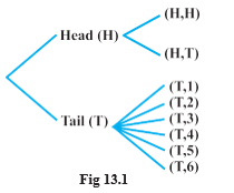
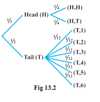
A card numbered from to is drawn. Given that its number is greater than , find the probability that it is even.
A die is thrown twice, and the sum is known to be . Find the conditional probability that a appeared at least once.
A coin is tossed. If it shows heads, toss it again; if it shows tails, roll a die. Find the probability that the die shows more than , given that at least one tail occurred.
Quick recap
- Conditional probability is , provided .
- Given , both the sample space and have conditional probability .
- The conditional addition rule subtracts the overlap; for disjoint events, add the probabilities directly.
- The conditional complement rule is .
- For equally likely outcomes, count favourable outcomes within the condition; otherwise use their actual probabilities.
- Always restrict the sample space to the given condition before calculating.
Multiplication Theorem on Probability
Multiplication Theorem
For events and , , using the conditional-probability form when the conditioning event has nonzero probability.
For three events, multiply each probability by the next event's probability conditional on all previous events.
Continue conditioning each event on the occurrence of all events before it.
Using the multiplication theorem
- Name the events in the order they occur.
- Find the probability of the first event.
- Find each later probability conditional on the earlier events.
- Multiply the probabilities to obtain the probability of their joint occurrence.
What is the probability that both drawn balls are black?
- An urn has 10 black and 5 white balls. Two balls are drawn without replacement. Find the probability that both are black.
- The probability that the first ball is black is:
- After a black ball is drawn, 9 black balls remain among 14 balls:
- Apply the multiplication theorem:
Do not use the first-draw probability again for a draw without replacement; the conditional probability changes because the contents of the urn change.
Three cards are drawn successively without replacement from a 52-card deck. Find the probability that the first two are kings and the third is an ace.
Independent Events
Use this test to decide whether two events are independent.
| Point | Independent | Mutually exclusive |
|---|---|---|
| Meaning | One event does not affect the probability of the other. | The events have no outcomes in common. |
| Intersection | May be nonempty. | and . |
| With positive probabilities | Cannot be mutually exclusive. | Cannot be independent. |
Events are mutually independent only if all three pairs are independent and the joint probability is also the product of all three individual probabilities.
For independent and , use the complement event that neither occurs.
If and are independent, then and , and , and and are also independent.
Testing independence
- Find the probabilities of each event.
- Find the probability that both events occur.
- Compare the joint probability with the product of the individual probabilities.
- Equal values mean independent events; unequal values mean dependent events.
Which of the pairs , and are independent?
- Three coins are tossed. Let be three heads or three tails, be at least two heads, and be at most two heads. Determine which pairs are independent.
- There are 8 equally likely outcomes. The event probabilities are:
- For and , their intersection contains only HHH, so the joint probability equals the product:
- For and , their intersection contains only TTT, so the probabilities are unequal:
- For and , the intersection has 3 outcomes, so the probabilities are unequal:
A die is thrown once. Let be the event of getting a multiple of 3 and the event of getting an even number. Are the events independent?
An unbiased die is thrown twice. Let mean an odd result on the first throw and an odd result on the second. Check independence.
If and are independent, show that and are independent.
Do not confuse independence with mutual exclusivity: mutual exclusivity concerns shared outcomes, while independence concerns probabilities. If both events have nonzero probabilities, mutually exclusive events are dependent.
Quick recap
- For two events, .
- For successive events, multiply each probability conditional on all previous events.
- Two events are independent exactly when .
- For three mutually independent events, test all three pairs and the triple intersection.
- Independence is different from mutual exclusivity; positive-probability mutually exclusive events are dependent.
- If two events are independent, their complements are also independent with the corresponding events.
- For independent and , .
Bayes' Theorem
Partition of a Sample Space
- Partition: Events form a partition of the sample space when they are pairwise disjoint, exhaustive, and each has nonzero probability.
- Example: Any nonempty event and its complement form a partition of the sample space.
Theorem of Total Probability
Use to find the overall probability of an event across all partition cases.
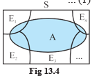
Bayes’ Theorem
For a partition and an event with , the conditional probability of hypothesis given equals its prior-weighted likelihood divided by the total probability of .
Applying Bayes’ theorem
- List the possible causes as a partition and identify the observed event.
- Write each cause’s prior probability and the probability of the observation under that cause.
- Multiply each prior by its corresponding likelihood and add the products to get the total probability of the observation.
- Divide the product for the required cause by the total probability of the observation.
What is the probability that a defective bolt was manufactured by machine B?
- Machines A, B and C make , and of a factory’s bolts. Their defective rates are , and . Given that a bolt is defective, find the probability it came from B.
- Let denote production by A, B and C, and let denote a defective bolt.
- Apply Bayes’ theorem to the hypothesis that machine B made the bolt.
- Evaluate the numerator and denominator.
Other Bayes’ theorem applications
- Two bags: Bag I has red and black balls; Bag II has red and black balls. With equal bag priors, the probability a red ball came from Bag II is .
- Three boxes: Choose one of three boxes equally: all gold, all silver, or one gold and one silver coin. Given a gold coin was drawn, the probability the other coin is gold is .
- Late doctor—transport priors: Train, bus, scooter and other transport have probabilities , respectively.
- Late doctor—late probabilities: The probabilities of being late by train, bus, scooter and other transport are , respectively.
- Late doctor—posterior: Given that he is late, the probability he came by train is .
Do not confuse (likelihood of the observation under a cause) with (probability of the cause after observing it); Bayes’ theorem converts the first into the second.
Random Variables
| Outcome | : number of heads | : heads minus tails |
|---|---|---|
A job has probability of a strike. It finishes on time with probability if there is a strike and if there is no strike. Find the probability it finishes on time.
A condition affects of a population. A test is positive for of affected people and for of unaffected people. Given a positive result, find the probability the person is affected.
A fair die is rolled. A person who tells the truth with probability reports that the result is six. Find the probability the roll was actually six.
Quick recap
- A partition consists of pairwise disjoint, exhaustive events with positive probabilities.
- Total probability adds the contributions of every partition case that can produce the event.
- Bayes’ theorem updates a cause’s prior probability after an observation.
- The denominator in Bayes’ theorem is the total probability of the observed event.
- Do not reverse conditional probabilities without applying Bayes’ theorem.
- A random variable assigns a real number to every sample-space outcome.
Miscellaneous Examples
Bayes’ Theorem: Identifying the Box
Bayes’ theorem — Bayes’ theorem finds the probability of a cause or source after an observed event has occurred.
Partition of a sample space — A set of events forms a partition when the events are pairwise disjoint and their union is the entire sample space.
If partition the sample space and , then . For , .
| Box | Black | White | Red | Blue |
|---|---|---|---|---|
| I | 3 | 4 | 5 | 6 |
| II | 2 | 2 | 2 | 2 |
| III | 1 | 2 | 3 | 1 |
| IV | 4 | 3 | 1 | 5 |
Set up the events
- Source events: Let mean box is selected; choosing uniformly gives for each box.
- Observed event: Let mean the drawn ball is black. Then , , , and .
Use the probability of drawing black from each box as the likelihood, weighted by the chance of choosing that box.
Applying Bayes’ theorem
- Define the possible sources and the observed event.
- Find each source probability and the conditional probability of the observation from that source.
- Multiply each source probability by its likelihood; divide the target source’s product by the sum of all products.
A box is chosen uniformly at random, and a ball drawn from it is black. Find the probability that the ball came from box III.
- The probability of a black ball from each box equals its black-ball count divided by its total.
- Apply Bayes’ theorem and cancel the equal box-selection probabilities.
Do not use only the likelihood as the answer; Bayes’ theorem must account for every possible box in the denominator.
Alternating Die Throws
Repeated-turn winning probability — When players alternate independent trials until success, a player’s possible winning events form a geometric series.
For first term and common ratio with , the infinite sum is .
For a fair die, let success be rolling a six and failure be not rolling a six. Each round consists of A’s throw followed by B’s throw.
Summing repeated winning chances
- Find the success and failure probabilities for one turn.
- Write the first few ways the player can win, including the failures before their winning turn.
- Identify the first term and common ratio, then sum the infinite geometric series.
- Use the complement for the other player if the game cannot end in a draw.
A and B alternately throw a die until one rolls a six. A starts. Find each player’s probability of winning.
- A wins on their first, third, fifth, and subsequent odd-numbered turns.
- This is a geometric series with first term and common ratio .
- Exactly one player eventually wins, so B’s probability is the complement.
A’s later winning chances require failures on both players’ earlier turns, so the common ratio is , not .
Bayes’ Theorem: Machine Setup
Posterior probability of a setup — The probability that a machine setup is correct after observing its output is found by weighting each setup’s likelihood by its prior probability.
Model the production information
- Prior probabilities: Correct setup has probability ; incorrect setup has probability .
- Likelihoods: Each item is acceptable with probability under and under ; for two independent items, the likelihoods are and .
Use independent-item probabilities to find the likelihood of the observed pair under each setup.
Using production evidence
- Assign prior probabilities to the possible setup states.
- Find the likelihood of the observed output under each state, using independence when appropriate.
- Apply Bayes’ theorem and simplify the posterior probability.
A machine is correctly set up with probability . It produces acceptable items with probability when correctly set up and otherwise. Given that two items are acceptable, find the probability the setup is correct.
- Let be the event that both produced items are acceptable; calculate the joint weights for the two setups.
- Divide the correct-setup weight by the total probability of the observed output.
For two acceptable items, use and as the likelihoods; do not use the single-item probabilities alone.
Conditional Probability: Chapter Toolkit
For , . Also, , , and .
For nonzero conditioning probabilities, . Events and are independent when ; equivalently, and whenever the conditional probabilities are defined.
Using the four-box data, find the probability that the drawn ball is black.
In the alternating die game, A starts and each player wins by rolling a six. Find the probability that B wins.
A machine is correctly set up with probability and incorrectly set up with probability . If two acceptable items are produced, find the posterior probability that the setup was incorrect.
Quick recap
- A partition consists of pairwise disjoint events whose union is the sample space.
- The total probability theorem adds the weighted likelihoods across a partition; Bayes’ theorem reverses the conditional probability.
- Given that the drawn ball is black, the probability it came from box III is .
- For alternating die throws with A starting, the winning probabilities are for A and for B.
- Given two acceptable items, the probability the machine was correctly set up is .
- Conditional probability, the multiplication rule, and independence connect joint and conditional events.
Formula sheet
Mathematics — ALL CHAPTERS
1
Relations And Functions
2
Inverse Trigonometric Functions
3
Matrices
4
DETERMINANTS
5
Continuity And Differentiability
6
Application Of Derivatives
7
Integrals
8
APPLICATION OF INTEGRALS
9
DIFFERENTIAL EQUATIONS
10
VECTOR ALGEBRA
11
Three Dimensional Geometry
12
Linear Programming
13
Probability
14
Proofs In Mathematics
15
Mathematical Modelling