Class 12 PCM . Mathematics . Mathematics Part II . Mathematical Modelling
Chapter 15: Mathematical Modelling
Ch 15
Mathematics
Class 12 PCM
Introduction
Meaning of Mathematical Modelling
General Modelling Process
- Identify the real-life question and the quantity to be found.
- Choose relevant variables, physical laws and suitable conditions or assumptions.
- Express the relationships mathematically and solve the resulting problem.
- Compare the mathematical result with practical values and interpret it in context.
Why can mathematical modelling be used to estimate pulse-crop yield?
- The problem is to estimate the yield of pulses from standing crops.
- The entire crop cannot be cut just to measure its yield.
- Use a mathematical model to estimate the yield without harvesting all the crop.
Why Mathematical Modelling Is Needed
| Problem | Why modelling is useful |
|---|---|
| Find the width of a river | Crossing the river may be difficult. |
| Find the best shot-put angle | The result can depend on thrower height, resistance of the medium and acceleration due to gravity. |
| Find the height of a tower | Reaching its top may not be possible. |
| Find the temperature at the Sun’s surface | It cannot be measured directly in an ordinary way. |
| Explain why heart patients may not be allowed to use a lift | The problem involves human physiology and physical conditions. |
| Find the mass of the Earth | It cannot be weighed directly. |
| Estimate pulse-crop yield | The entire crop cannot be cut just to measure its yield. |
| Estimate the volume of blood in a person | The entire blood supply cannot be removed for measurement. |
| Estimate India's population in 2020 | An estimate is needed without waiting until that year. |
Why can crop yield be estimated using modelling instead of harvesting the entire crop?
Why is mathematical modelling useful for estimating a future population?
Quick recap
- Mathematical modelling represents a real-life situation using mathematics and suitable conditions.
- Models may be expressed in words, drawings, programs or formulae.
- A model focuses on the parts of a situation relevant to the question.
- Physical insight and appropriate laws or assumptions help build a useful model.
- Interpret the mathematical result and compare it with practical values.
- Modelling helps estimate or solve problems that are difficult to measure directly.
Principles of Mathematical Modelling
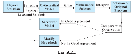
Principles and modelling cycle
Modelling cycle
- Identify the real situation
- Formulate a model using variables, assumptions and known laws
- Solve the mathematical problem
- Interpret and compare the result with observations
- Accept if suitable; otherwise revise assumptions and reformulate
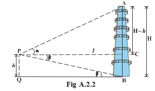
Estimating a tower’s height
Tower-height model — The tower’s height can be found from an observer’s eye height, horizontal distance and angle of elevation.
Model setup
- Variables: Let tower height be , observer’s eye height be , horizontal distance be , and angle of elevation be .
- Geometry: The vertical difference between the tower top and the observer’s eye is .
- Accessible base: Use the tangent ratio to calculate the height above the observer’s eye, then add .
- Inaccessible base: If is unknown, measure the angle of depression to the tower’s foot; then .
Use the first relation when the horizontal distance is known; use the second when the tower’s foot is inaccessible.
Find the tower’s height from the given measurements.
- Suppose the observer’s eye is m above the ground, the tower is m away, and the angle of elevation is .
- Apply the tower-height model.
- Substitute the measurements and evaluate.
Matrices for production and raw-material requirements
Production matrix model — Matrix multiplication combines client orders with per-unit material requirements to calculate total raw materials needed.
Matrix meanings and dimensions
- Order matrix : Rows represent clients and columns represent products; each entry is the quantity ordered.
- Material matrix : Rows represent products and columns represent raw materials; each entry is the material needed per unit of product.
- Total requirement : Rows represent clients and columns represent raw materials; each entry gives material required for that client’s order.
- Dimensions: If there are clients, products and materials, then is , is , and is .
The product is defined because the number of columns of equals the number of rows of .
Can the firm fulfil both orders with units of , of , and of ?
- Use the client-order matrix and per-unit material matrix shown below.
- Multiply each client’s product quantities by the corresponding material requirements.
- Add the two clients’ requirements and compare with availability.
Revising orders
- Reduced orders: For , the requirements are .
- Totals: The revised orders need units of , of , and of , so they fit within the available quantities.
- Further improvement: Orders can be adjusted again to use more of the available stock, if that is the firm’s goal.
Choosing production to use available materials
Resource-use model — A system of linear equations can determine production quantities that use specified amounts of several raw materials.
For products made in quantities , respectively, set each material’s total use equal to its available amount.
How many units of each product use all the available materials?
- Write the material-balance system in matrix form.
- Solve the simultaneous equations, for example by elementary row operations.
- Check the quantities against all three material totals.
Production planning with a profit objective
Linear programming model — A linear programming model maximizes or minimizes a linear objective while satisfying linear constraints.
Medicine production model
- Variables: Let and be the numbers of bottles of medicines and .
- Profit: Profit per bottle is Rs. for and Rs. for .
- Constraints: Raw materials allow at most bottles of and of ; bottle capacity is total.
- Preparation time: Filling bottles takes hours for and hour for ; hours are available.
Maximize profit over the feasible region, the set of points satisfying every constraint.
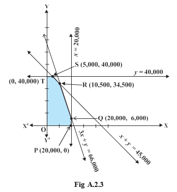
Corner-point method
- Form the objective function and list all constraints.
- Identify the vertices of the feasible region.
- Evaluate the objective function at every vertex; choose the greatest value for a maximization problem.
What production plan gives the maximum profit?
- Use the feasible-region vertices and evaluate the profit at each.
- Evaluate the remaining vertices.
- Select the feasible vertex with the greatest profit.
A cost–income–profit model
Break-even model — A break-even model compares sales income with fixed and variable production costs to determine when profit is zero.
Assumptions and variables
- Assumptions: Fixed cost does not depend on output; variable cost is directly proportional to output; all units produced are sold at one fixed price.
- Variables: is units produced and sold; , , and are total cost, income, and profit.
- Parameters: is fixed cost, is variable cost per unit, and is selling price per unit.
The break-even formula assumes . Positive profit requires output above break-even; the marginal profit per extra unit is .
Find the break-even number of units.
- Suppose fixed cost is Rs. , variable cost is Rs. per unit, and selling price is Rs. per unit.
- Set profit equal to zero and solve for output.
- Check the result using income and cost at that output.
Salt concentration in a stirred tank
Mixing model — A differential equation models the changing amount of salt by subtracting the salt outflow rate from the salt inflow rate.
Tank data and rate balance
- Initial salt: The tank holds L at g/L, so it initially contains kg of salt.
- Inflow: Brine at g/L enters at L/min, bringing in kg/min of salt.
- Outflow: Since the mixture is uniform, its salt concentration at time is kg/L; the salt leaves at kg/min.
- Volume: Inflow and outflow rates are equal, so tank volume stays at L.
Here is salt amount in kilograms and is time in minutes. The initial condition determines the integration constant.
How much salt is in the tank at any time after the flow begins?
- Let be the salt amount, in kilograms. Write the rate as inflow minus outflow.
- Solve the linear differential equation.
- Use the initial amount to find the constant.
- State the amount at time and its limiting value.
For a finite time after flow starts, the salt amount satisfies .
A client orders units of and units of . Each unit of requires units of materials and each unit of requires . Find the total material requirements.
A product uses units of material and units of per unit. If available amounts are and , how many units use both materials completely?
A firm has fixed costs of Rs. , variable cost Rs. per unit, and selling price Rs. per unit. Find the break-even output.
Quick recap
- A model starts with the question, relevant data, variables, assumptions and governing laws.
- Solve the mathematical model, interpret the result, and compare it with observations; revise if it fails.
- For orders and per-unit material requirements, the matrix product gives total materials required.
- Material-balance equations can determine production quantities that use available stock.
- Linear programming maximizes or minimizes an objective over the feasible region; test its vertices.
- With fixed and variable costs, profit is and break-even output is when .
- For a well-stirred tank, salt change equals inflow rate minus outflow rate; the example approaches kg.
Limitations of Mathematical Modelling
Mathematical modelling — Using mathematics to represent and study real-world situations.
Uses and limits
Where modelling is used—and why it can be difficult
- Successful applications: Modelling is widely used in mathematical physics, mathematical economics, operations research and bio-mathematics.
- Unmodelled situations: Some situations are too complex to model, or the models formed are mathematically intractable—that is, too difficult to handle mathematically.
- Computing advances: Powerful computers and supercomputers have enabled modelling of many more situations, including complex ones.
- More realistic models: Faster, advanced computers make it possible to build models that are more realistic and agree better with observations.
Choosing and estimating parameters
A key modelling challenge
- Parameter choice: There are no good general guidelines for choosing the variables or parameters in a model.
- Parameter estimation: Finding accurate values for the chosen variables or parameters is also difficult.
- Too many parameters: Five or six parameters may produce a reasonably accurate fit, but a good fit alone does not establish that the model is reliable.
- Keep the model minimal: Use the fewest parameters needed so their values can be estimated accurately.
Why is it not enough to judge a model only by how well it fits the observations?
- Suppose a model uses five or six parameters to fit a set of observations.
- The fit may be good, but let mean a good fit and mean a reliable model; the fit alone does not guarantee reliability.
- If a smaller number is sufficient, prefer the minimum number of parameters that still models the situation adequately.
Large and complex models
Scale and collaboration
- Examples: Large or complex modelling problems arise in world models of the environment, oceanography and pollution control.
- Teamwork: These challenges involve modellers from mathematics, computer science, physics, engineering, social sciences and other disciplines.
Give two reasons why some real-world situations remain unmodelled.
How have powerful computers helped modelling, and what difficulty remains?
Quick recap
- Modelling is used in mathematical physics, economics, operations research and bio-mathematics.
- Some situations are too complex, while some models are mathematically intractable.
- Advanced computers enable more complex, realistic models with better agreement with observations.
- Choosing variables or parameters and estimating their values accurately remain difficult.
- A good fit using five or six parameters does not guarantee reliability; use the fewest necessary parameters.
- Large-scale problems such as environmental modelling, oceanography and pollution control require multidisciplinary collaboration.
Formula sheet
Mathematics — ALL CHAPTERS
1
Relations And Functions
2
Inverse Trigonometric Functions
3
Matrices
4
DETERMINANTS
5
Continuity And Differentiability
6
Application Of Derivatives
7
Integrals
8
APPLICATION OF INTEGRALS
9
DIFFERENTIAL EQUATIONS
10
VECTOR ALGEBRA
11
Three Dimensional Geometry
12
Linear Programming
13
Probability
14
Proofs In Mathematics
15
Mathematical Modelling