Class 11 Humanities . Economics . Statistics For Economics . Correlation
Chapter 6: Correlation
Ch 6
Economics
Class 11 Humanities
Introduction
Introduction to Correlation
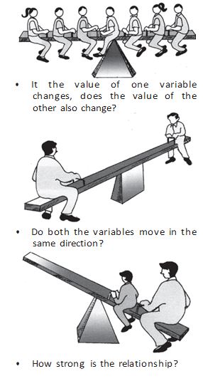
Correlation analysis — A method for examining systematically whether and how two variables are related.
Examples of relationships
- Temperature and visitors: Rising summer temperatures are associated with more visitors at hill stations.
- Temperature and ice-cream sales: Ice-cream sales tend to rise as temperatures increase.
- Tomato supply and price: When supply rises, prices may fall—for example, from Rs. 40 per kg to Rs. 4 per kg or less.
Types of Relationships
| Type | Meaning | Example |
|---|---|---|
| Cause-and-effect relationship | One variable may influence or help explain changes in another. | Low rainfall may be associated with low agricultural productivity. |
| Coincidental relationship | Two variables change together, but there is no meaningful cause-and-effect explanation. | Migratory birds arriving at a sanctuary and local birth rates; shoe size and money in a person's pocket. |
| Relationship due to a third variable | A third factor affects both variables, making them appear related. | Temperature increases both ice-cream sales and swimming-pool use, which may increase drowning deaths. |
A third variable can create an apparent relationship
- Higher temperature → more ice-cream sales.
- Higher temperature → more people swim to cool off → more opportunities for drowning deaths.
- Ice-cream sales and drowning deaths may therefore be correlated, even though eating ice cream does not cause drowning.
What Correlation Measures
Correlation — A measure of the direction and intensity (strength) of the relationship between variables.
Core ideas
- Covariation: Correlation describes how variables change in relation to one another.
- Not causation: A correlation does not, by itself, prove that one variable causes a change in another.
- Direction: When one variable changes, the other tends to change in the same direction or the opposite direction.
- Linear assumption: In this chapter, an existing relationship is treated as linear—its relative movement can be represented by a straight line on a graph.
Do not interpret correlation as proof of cause and effect; coincidence or the influence of a third variable may explain the relationship.
Positive and Negative Correlation
| Positive correlation | Negative correlation | |
|---|---|---|
| Direction of movement | Variables move in the same direction. | Variables move in opposite directions. |
| When one variable rises | The other tends to rise too. | The other tends to fall. |
| When one variable falls | The other tends to fall too. | The other tends to rise. |
| Examples | Income and consumption; temperature and ice-cream sales. | Apple price and quantity demanded; study time and chances of failing. |
- Correlation
- The direction and strength of a relationship between variables.
- Covariation
- The way two variables change in relation to one another.
- Positive correlation
- A relationship in which variables move in the same direction.
- Negative correlation
- A relationship in which variables move in opposite directions.
What does correlation measure, and what does it not prove?
Distinguish positive from negative correlation.
Quick recap
- Correlation analysis examines how two variables are related.
- A relationship may reflect cause and effect, coincidence, or the influence of a third variable.
- Correlation measures the direction and intensity of covariation, not causation.
- Positive correlation means variables move in the same direction.
- Negative correlation means variables move in opposite directions.
- The relationships considered here are assumed to be linear.
Techniques For Measuring Correlation
Main Techniques
| Technique | What it shows |
|---|---|
| Scatter diagram | Visual direction and closeness of association; gives no numerical value. |
| Karl Pearson’s coefficient | Numerical measure of the direction and degree of a linear relationship between two variables. |
| Spearman’s rank correlation | Measures linear association between ranks assigned to items according to their attributes. |
Linear relationship — A relationship that can be represented by a straight line.
Attributes — Qualities that cannot be measured numerically, such as intelligence, physical appearance and honesty.
Scatter Diagram
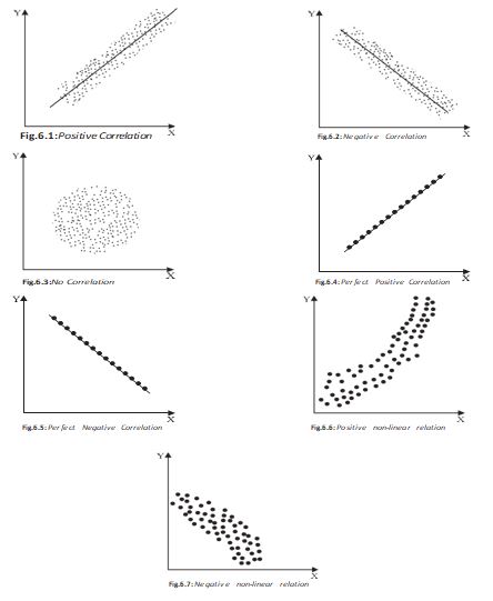
Scatter diagram — A graph of paired values of two variables, plotted as points to assess their relationship visually without calculating a numerical measure.
Reading the pattern
- Direction is shown by the overall trend; closeness of points indicates the strength of the relationship.
- Positive correlation: points trend upward; as rises, tends to rise.
- Negative correlation: points trend downward; as rises, tends to fall.
- No correlation: points show no clear upward or downward trend.
- Perfect correlation: all points lie exactly on a straight line; it may be perfectly positive or perfectly negative.
- Linear pattern: points lie on or close to a straight line; a curved pattern is non-linear.
Karl Pearson’s Coefficient of Correlation
Karl Pearson’s coefficient — A precise numerical measure of the direction and degree of the linear relationship between two variables; also called the product-moment or simple correlation coefficient.
Means, deviations and covariance
- Means: For paired observations, and .
- Deviations: Let and ; these are deviations from the respective means.
- Variance: ; similarly for .
- Standard deviation: and are the positive square roots of the respective variances.
- Covariance: ; its sign determines the sign of .
Use for paired observations; and .
Use when the sums of raw values, squares and cross-products are available.
Use Pearson’s coefficient only after checking that the relationship is linear. For a non-linear pattern, the coefficient can be misleading.
Properties and Interpretation of
- Range: . A calculated value outside this range signals an error.
- No units: is a pure number; its value does not include the units of measurement.
- Sign: means the variables move in the same direction; means they move in opposite directions.
- Strength: Values near or show a strong linear relationship; values near show a weak linear relationship.
- Zero: means no linear relationship, although a non-linear relationship may exist.
- Perfect relationship: or indicates an exact linear relationship.
- Origin and scale: Changing origin and scale does not change when the scale factors are of the same sign.
If are assumed means and are common scale factors of the same sign, the transformed variables have the same correlation as the originals.
Examples and interpretation
- Positive examples: A rise in coffee prices may increase demand for tea; better irrigation may raise yield; higher temperatures may increase ice-cream sales.
- Negative examples: A rise in a commodity’s price may lower its demand; higher interest rates may reduce demand for funds.
- Context matters: Deaths and doctors sent to villages may be positively correlated because doctors are sent to the worst-affected places; some deaths may be terminal or unrelated to the epidemic.
- Delayed effects: Doctors’ benefits may appear later, and events such as a tsunami can increase deaths independently of the epidemic.
- English and Statistics marks: shows weak positive association, while shows strong positive association.
- Vegetable supply and price: indicates a stronger inverse relationship than ; a large supply may not lower price if transport sends it to other markets.
| Years of schooling () | Yield per acre in '000 Rs. () |
|---|---|
| 0 | 4 |
| 2 | 4 |
| 4 | 6 |
| 6 | 10 |
| 8 | 10 |
| 10 | 8 |
| 12 | 7 |
Example calculation: farmer education and yield
- Means: For the seven pairs, and .
- Deviation totals: , and .
- Result: ; education and yield are positively correlated, with a fairly strong linear association.
Step Deviation Method
Step deviation method — A shortcut for calculating correlation by transforming large values with assumed means and common factors; the correlation remains unchanged.
Calculate correlation using transformed values
- Choose assumed means and convenient scale factors ; transform each paired observation.
- Calculate , , , , and the number of pairs .
- Substitute the transformed sums in the shortcut formula; this gives the original correlation.
| 2 | 1 | 4 | 1 | 2 |
| 5 | 3 | 25 | 9 | 15 |
| 9 | 8 | 81 | 64 | 72 |
| 12 | 10 | 144 | 100 | 120 |
| 13 | 13 | 169 | 169 | 169 |
| Totals: |
For the five price-index and money-supply pairs, the transformed sums give a strong positive relationship.
- Interpretation: Price index and money supply have a strong positive correlation; an increase in money supply is associated with a rise in the price index.
When should Karl Pearson’s coefficient be used?
What does mean?
Quick recap
- Scatter diagrams show direction and closeness visually but give no numerical coefficient.
- Karl Pearson’s coefficient measures the direction and strength of a linear relationship.
- The sign of shows direction; its magnitude shows strength, and .
- A zero Pearson coefficient means no linear association, not necessarily no relationship of any kind.
- Check the scatter diagram and interpret correlations in context before drawing conclusions.
- The step deviation method simplifies calculations without changing the correlation.
Spearman’s rank correlation
Meaning and uses
Spearman’s rank correlation — A measure of linear association between the ranks assigned to observations, rather than between their original values.
When it is useful
- Origin: Developed by British psychologist C.E. Spearman.
- Unmeasurable values: Use ranks when measurements are unavailable, such as ranking students by height and weight without instruments.
- Relative qualities: Use it for qualities such as fairness, honesty or beauty when at least one variable can only be judged relatively.
- Clear-direction non-linear relationships: It can be used in some cases where the direction of association is clear but the relationship is non-linear.
- Extreme values: It is not affected by extreme values, making it useful in such data and, in this respect, preferable to Karl Pearson’s coefficient.
Formula and interpretation
- Calculation idea: Replace each observation with its rank, then compare the paired ranks for the two variables.
- Rank difference (): The difference between the ranks assigned to the same observation for the two variables.
- Interpretation: Like the simple correlation coefficient, it indicates the direction and degree of association; here, the association is between ranks.
- Range: The coefficient lies between and .
- Limitation: It is generally less accurate than the ordinary method because ranking does not use all the information in the original data.
Use for observations; is the difference between the paired ranks.
Relation to the simple correlation coefficient
- First differences: Differences between consecutive values after arranging the series in order of magnitude.
- Usual pattern: First differences are almost never constant; values often cluster around the centre, where differences tend to be smaller.
- If first differences were constant: The simple correlation coefficient and rank coefficient would give identical results.
- General relation: In general, is less than or equal to .
Quick recap
- Spearman’s rank correlation measures linear association between ranks, not the original values.
- It is useful for unmeasurable or relative qualities, some clear-direction non-linear relationships, and data with extreme values.
- Its formula is , where is the paired rank difference and is the number of observations.
- It ranges from to and has the same general interpretation as the simple correlation coefficient.
- It usually uses less information and is less accurate than the ordinary method; in general, .
Calculation of Rank Correlation Coefficient
Spearman’s rank correlation coefficient — A measure of the direction and strength of the linear relationship between two variables using their ranks.
Case 1: Ranks are given
Here, is the difference between paired ranks and is the number of pairs.
| Judge | Competitor 1 | Competitor 2 | Competitor 3 | Competitor 4 | Competitor 5 |
|---|---|---|---|---|---|
| A | 1 | 2 | 3 | 4 | 5 |
| B | 2 | 4 | 1 | 5 | 3 |
| C | 1 | 3 | 5 | 2 | 4 |
Comparing judges’ rankings
- Compare pairs: Three judges produce three possible pairs; calculate rank correlation for each pair.
- A and B: , ; therefore .
- A and C: , ; therefore .
- B and C: The listed ranks give , so .
- Conclusion: A and C have the closest rankings because their coefficient, , is the largest.
The source states that the B–C coefficient is , but the listed rankings produce . Applying the formula to the given ranks shows that the stated value is inconsistent with the data.
Case 2: Ranks are not given
Rank the data, then calculate
- Rank each variable separately, using the same convention for both; in this example the highest mark receives rank 1.
- For each student, find the difference between the two ranks and square it.
- Substitute and into Spearman’s formula.
| Student | Statistics marks | Economics marks | Statistics rank | Economics rank |
|---|---|---|---|---|
| A | 85 | 60 | 1 | 1 |
| B | 60 | 48 | 4 | 5 |
| C | 55 | 49 | 5 | 4 |
| D | 65 | 50 | 3 | 3 |
| E | 75 | 55 | 2 | 2 |
Students’ example result
- Rank differences: Only students B and C have non-zero differences; each has , so .
- Coefficient: For , .
Case 3: Ranks are repeated
Assigning tied ranks
- Common rank: Give tied values the average of the rank positions they would have occupied.
- Next rank: After a tie, continue with the next rank after all positions used by the tied values.
- Example: Three equal values spanning ranks 9, 10 and 11 each receive rank .
For each tied group, is the number of repeated values. Add every group’s correction factor to .
Example with repeated values
- Tied groups in : The value occurs three times, while and each occur twice.
- Correction factors: For these groups, the factors are , , and ; total correction is .
- Rank differences: The rank table gives and .
- Coefficient: .
- Interpretation: and have a positive but not strong rank relationship.
Choosing and interpreting correlation
| Point | Karl Pearson’s coefficient | Spearman’s rank coefficient |
|---|---|---|
| Basis | Measured variable values | Ranks of the values |
| Use | Numerically measured variables | Variables that cannot be measured precisely or are expressed as ranks |
| Relationship measured | Linear relationship | Linear relationship using ranks |
What correlation tells us
- Scatter diagram: Gives a visual presentation of the nature of a relationship and is not limited to linear relationships.
- Correlation coefficients: Karl Pearson’s coefficient and Spearman’s rank coefficient measure linear relationships numerically.
- Interpretation: Correlation indicates the direction and intensity of change associated with another variable; it does not establish causation.
- Rank method: Rank both variables consistently; when ranks tie, use average ranks and include all required correction factors.
- Correlation is not causation: It shows that variables vary together, not that one causes the other.
Quick recap
- Spearman’s coefficient measures direction and strength of a relationship using ranks.
- With no ties, calculate rank differences, square them and apply the rank-correlation formula.
- When ranks are missing, rank each variable first using a consistent order.
- Tied values receive the average of the rank positions they occupy.
- Add a correction factor for every tied group when ranks are repeated.
- Scatter diagrams show relationships visually; correlation does not establish causation.
Economics — ALL CHAPTERS
1
Introduction
2
Theory of Consumer Behaviour
3
Production And Costs
4
The Theory Of The Firm Under Perfect Competition
5
Market Equilibrium
1
Introduction
2
Collection of Data
3
Organizing of Data
4
Presentation of Data
5
Measures of Central Tendency
6
Correlation
7
Index Numbers
8
Use of Statistical Tools