Class 11 Humanities . Economics . Introductory Micro Economics . Production and Costs
Chapter 3: Production And Costs
Ch 3
Economics
Class 11 Humanities
Introduction & Production Function
Production and the Firm
Production — The process by which a firm transforms inputs into output.
The firm and its objective
- Inputs: Firms use resources such as labour, land, capital, machines and raw materials to produce goods or services.
- Examples: A farmer combines land, labour, seeds and equipment to produce wheat; a domestic helper uses labour to provide cleaning services.
- Assumptions: This introductory model treats production as instantaneous and often uses “production” and “supply” interchangeably.
- Cost and revenue: A firm pays for inputs, creating production costs; selling output earns revenue.
- Profit: Profit is revenue minus cost. The firm is assumed to aim for the maximum possible profit.
Revenue remaining after production costs are subtracted.
Production Function
Production function — A relationship showing the maximum output a firm can produce from different combinations of inputs.
Core features
- Inputs and output: The simplified model uses labour () and capital () to produce output ().
- Maximum output: For each input combination, the function gives the greatest output achievable; using inputs efficiently means no more output can be obtained from those same inputs.
- Technology: A production function is defined for a given technology. Improved technology raises the maximum output possible from input combinations and creates a new production function.
- Input changes: In the examples here, increasing either input raises output; if either necessary input is zero, production is zero.
is maximum output; is labour and is capital.
A simple farmer example uses land and labour; if land is hectare and labour is hours per day, the illustrative function gives tonnes.
| Labour () | Capital () | Maximum output () |
|---|---|---|
| 1 | 1 | 1 |
| 2 | 2 | 10 |
| 3 | 2 | 18 |
Do not treat as the general production function: it is only one illustrative example. In general, write .
Isoquants
Isoquant — A curve representing all combinations of two inputs that can produce the same maximum output.
Reading isoquants
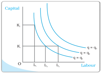
- Axes: Labour () is shown on the horizontal axis and capital () on the vertical axis.
- Output levels: Each isoquant is labelled by its output level; points on one curve produce the same maximum output.
- Example: Output can be produced by , or .
- Output of 50: From the numerical table, occurs at , and .
- Higher output: Holding capital at , increasing labour from to can move production to a higher isoquant.
- Negative slope: With positive marginal products, increasing one input allows the same output to be maintained with less of the other input.
- Factors of production
- Inputs used by a firm to produce output.
- Technology
- The productive knowledge determining the maximum output possible from input combinations.
- Efficient production
- Production where no greater output can be obtained from the same quantity of inputs.
- Isoquant
- A curve of input combinations that produce the same maximum output.
What does a production function show?
Why are isoquants negatively sloped when both inputs have positive marginal products?
Quick recap
- Production transforms inputs into output; firms seek maximum profit, calculated as revenue minus cost.
- A production function gives maximum output from input combinations for a given technology.
- The two-input model represents output as , where is labour and is capital.
- Improved technology can raise maximum output and results in a new production function.
- An isoquant joins input combinations that produce the same maximum output; output occurs at , and in the table.
- With positive marginal products, isoquants slope downward.
The Short Run And The Long Run
Short Run and Long Run
Short run — A period in which at least one factor of production is fixed, so the firm can vary output by changing only its variable factor.
Factors in the short run
- Fixed factor: An input the firm cannot change during the short run.
- Variable factor: An input the firm can change to alter output.
- Example: If capital is fixed at 4 units, the firm can vary labour to produce different output levels.
Long run — A period in which all factors of production can be varied; therefore, there is no fixed factor.
| Point | Short Run | Long Run |
|---|---|---|
| Inputs | At least one input is fixed; others may vary. | All inputs can vary. |
| Output changes | Achieved by changing the variable input(s). | Achieved by changing one or more inputs. |
| Time period | Not defined by a set number of days, months, or years. | Usually longer than the short run for the same production process; duration varies by process. |
Classify a period by whether inputs can be changed—not by its calendar length.
Total, Average and Marginal Product
Total Product (TP) — The output produced by different quantities of one variable input while all other inputs are held constant.
Total Product
- Other names: Total return or total physical product of the variable input.
- Example: With capital fixed at 4 units, the outputs corresponding to each labour level form the total product of labour schedule.
Average Product (AP) — Output per unit of the variable input.
Use output divided by the quantity of labour.
Marginal Product (MP) — The change in output per unit change in an input, with all other inputs held constant.
For labour changing by one unit, MP is the difference between the two successive total-product levels.
Product Relationships
- Successive-unit MP: For a one-unit increase in labour, subtract the previous TP from the new TP.
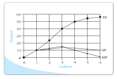
- Example: When labour rises from 1 to 2, TP rises from 10 to 24; therefore, the second worker's MP is 14.
- Total product: The sum of the marginal products of all units employed equals TP.
- Average product: AP at any employment level is the average of the marginal products up to that level.
- At zero input: MP is undefined because inputs cannot take negative values.
- Other names: AP and MP are also called average and marginal returns to the variable input.
| Labour (L) | TP | MPₗ | APₗ |
|---|---|---|---|
| 0 | 0 | — | — |
| 1 | 10 | 10 | 10 |
| 2 | 24 | 14 | 12 |
| 3 | 40 | 16 | 13.33 |
| 4 | 50 | 10 | 12.5 |
| 5 | 56 | 6 | 11.2 |
| 6 | 57 | 1 | 9.5 |
Diminishing Marginal Product and Variable Proportions
Law of Variable Proportions (Law of Diminishing Marginal Product) — When one input is increased while another is fixed, its marginal product initially rises, but after a certain employment level it begins to fall.
How Product Changes
- TP: Increases as more of the variable input is used, but its rate of increase changes.
- MP: Shows the rate of change in TP; it rises at first and later falls.
- Table example: MP rises from 10 to 16 as labour increases from 1 to 3, then falls with further labour additions.
- Factor proportions: The ratio in which two inputs are combined in production.
Why Marginal Product First Rises and Then Falls
- One factor is fixed while the variable factor increases.
- Initially, the input combination becomes more suitable for production.
- Each additional unit contributes more output, so marginal product rises.
- Beyond a certain employment level, the variable input crowds the fixed factor.
- Inputs become less efficient to use together, so each added unit contributes less and marginal product falls.
Illustration: Labour and Fixed Land
- Initial stage: With 4 hectares of land and only one worker, land is underused; adding workers lets the land be cultivated more effectively.
- Later stage: As more workers share the same land, it becomes crowded and each worker has less land to work efficiently.
- Result: The extra output from each additional worker first rises and then falls.
- Fixed factor
- An input that cannot be varied in the short run.
- Variable factor
- An input that can be changed in the short run.
- Total product
- Total output from a variable input, with other inputs fixed.
- Marginal product
- Additional output per unit change in an input.
- Factor proportions
- The ratio in which two inputs are combined.
Distinguish between the short run and the long run.
Define average product and marginal product.
State the law of variable proportions and explain why marginal product eventually falls.
Quick recap
- Short run: at least one factor is fixed; long run: all factors are variable.
- The short run and long run are defined by input flexibility, not a set calendar duration.
- TP measures output; AP is output per unit of input; MP is the change in output per unit change in input.
- TP equals the sum of marginal products; AP is the average of marginal products up to that input level.
- With one factor fixed, MP initially rises as proportions improve, then falls as the variable factor crowds the fixed factor.
Shapes Of Total Product, Marginal Product And Average Product Curves
Total Product, Marginal Product and Average Product
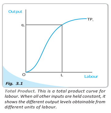
Marginal Product (MP)
- MP: The additional output produced by using one more unit of an input.
- Law of variable proportions: With other inputs fixed, MP initially rises and then falls as more of the variable input is employed.
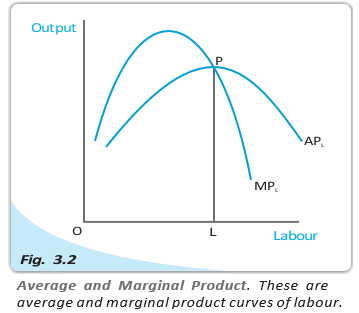
- Shape: The MP curve is typically inverse U-shaped.
Average Product (AP) and its relation to MP
- AP: Output per unit of the input; for the first unit of the variable input, MP and AP are equal.
- While MP > AP: AP rises, because the additional product is above the current average.
- When MP < AP: AP falls, because the additional product is below the current average.
- Intersection: MP cuts AP from above at AP's maximum; AP rises to the left of this point and falls to its right.
- Shape: The AP curve is inverse U-shaped.
Returns to Scale
For and , compare output after scaling both inputs with times the original output.
Output comparison
- CRS: .
- IRS: .
- DRS: .
- Example: If both inputs double, doubled output means CRS; less than doubled means DRS; more than doubled means IRS.
Costs
- Least-cost choice: A firm chooses the least expensive input combination capable of producing its desired output, given factor prices.
- Cost function: It gives the least cost of producing each output level, given factor prices and technology.
Cobb–Douglas Production Function
- Total product (TP)
- Total output produced using a given amount of input.
- Marginal product (MP)
- Additional output from one more unit of input.
- Average product (AP)
- Output per unit of input.
- Returns to scale
- How output changes when all inputs change in the same proportion.
Why does AP rise when MP is greater than AP?
How does the Cobb–Douglas function's returns to scale depend on its exponents?
Quick recap
- TP rises as the variable input increases while other inputs are fixed.
- MP first rises and then falls; its typical curve is inverse U-shaped.
- AP rises when MP exceeds AP and falls when MP is below AP; MP crosses AP at AP's maximum.
- Returns to scale compare the proportional change in output with the common proportional change in all inputs.
- The cost function identifies the least cost of producing each output level.
- For a Cobb–Douglas function, the sum determines returns to scale.
Short Run Costs
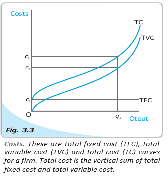
Types of Short-Run Costs
Use this to find total cost at any output level.
| Output (units) | TFC (Rs.) | TVC (Rs.) | TC (Rs.) | AFC (Rs.) | AVC (Rs.) | SAC (Rs.) | SMC (Rs.) |
|---|---|---|---|---|---|---|---|
| 0 | 20 | 0 | 20 | — | — | — | — |
| 1 | 20 | 10 | 30 | 20 | 10 | 30 | 10 |
| 2 | 20 | 18 | 38 | 10 | 9 | 19 | 8 |
| 3 | 20 | 24 | 44 | 6.67 | 8 | 14.67 | 6 |
| 4 | 20 | 29 | 49 | 5 | 7.25 | 12.25 | 5 |
| 5 | 20 | 33 | 53 | 4 | 6.6 | 10.6 | 4 |
| 6 | 20 | 39 | 59 | 3.33 | 6.5 | 9.83 | 6 |
| 7 | 20 | 47 | 67 | 2.86 | 6.7 | 9.57 | 8 |
| 8 | 20 | 60 | 80 | 2.5 | 7.5 | 10 | 13 |
| 9 | 20 | 75 | 95 | 2.22 | 8.33 | 10.55 | 15 |
| 10 | 20 | 95 | 115 | 2 | 9.5 | 11.5 | 20 |
Reading the cost schedule
- At zero output: The firm still incurs TFC, so TC equals Rs. 20; TVC is zero.
- As output increases: TC equals the corresponding TFC plus TVC; for example, at , TC is Rs. 20 + Rs. 18 = Rs. 38.
- Cost changes: With TFC fixed, any change in TC as output changes comes entirely from a change in TVC.
Average and Marginal Costs
The identity follows because total cost is the sum of fixed and variable costs.
Marginal cost
- Short-run marginal cost (SMC): The increase in total cost per additional unit of output.
- Since TFC is fixed: The increase in TC is entirely the increase in TVC, so SMC measures the additional TVC from producing extra output.
- At zero output: SMC is undefined; it requires a change in output to calculate.
- Cumulative link: Adding marginal costs up to a given output gives the TVC at that output. AVC is the average of marginal costs up to that output.
Here, means change; for one-unit output steps, SMC is the change in TC between successive output levels.
Example: marginal cost at the fifth unit
- Change in TC: At , TC rises from Rs. 49 at to Rs. 53.
- Calculation: and , so SMC is Rs. 4.
Shapes of Short-Run Cost Curves
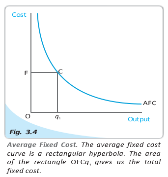
Average fixed cost (AFC)
- As output rises: AFC falls because a fixed total cost is spread over more units.
- Curve shape: AFC is a rectangular hyperbola: it becomes very large as output approaches zero and tends towards zero as output grows.
- Constant product: At every positive output, .
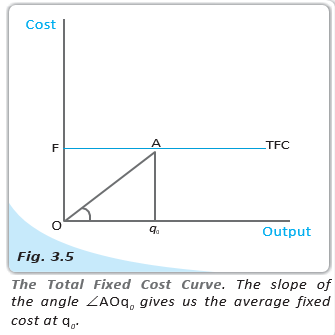
AFC from the total fixed cost curve
- Geometric meaning: At output , AFC equals TFC divided by output; on the graph this is the slope from the origin to the TFC point.
- If the line makes angle with the output axis: .
Short-run marginal cost (SMC)
- Why SMC first falls: Under the law of variable proportions, marginal product initially rises, so fewer additional inputs are needed for each extra unit of output.
- Why SMC later rises: After marginal product begins to fall, more additional inputs are needed per extra unit; with factor prices given, marginal cost rises.
- Curve shape: SMC is U-shaped: it falls initially and rises after reaching a minimum.
- Area relation: TVC at an output level equals the area under the SMC curve up to that output.
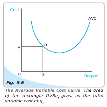
Average variable cost (AVC)
- Beginning: For the first unit, SMC and AVC are equal, so the curves start together.
- When SMC falls: AVC also falls, but less quickly because AVC averages costs across units.
- When SMC rises: AVC keeps falling while SMC is below AVC; once SMC rises above AVC, AVC begins to rise.
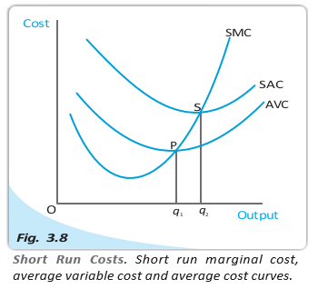
- Curve shape and intersection: AVC is U-shaped. SMC crosses AVC from below at AVC's minimum point.
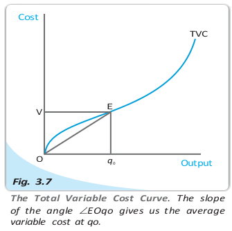
- Geometric meaning: At output , AVC is the slope of the line from the origin to the corresponding point on the TVC curve; TVC is also .
SAC and the Relationship Between Average and Marginal Costs
- TFC is constant; at zero output, TC equals TFC.
- SMC crosses AVC and SAC from below at each curve's minimum.
- SAC = AVC + AFC, so SAC lies above AVC by the amount of AFC.
Quick recap
- Short-run costs divide into fixed cost and variable cost: .
- Average costs are per-unit costs; .
- SMC is the change in total cost per change in output; with fixed TFC, it reflects the change in TVC.
- TFC stays constant, while TVC and TC rise with output; AFC declines as output increases.
- SMC, AVC and SAC are U-shaped, and SMC crosses each average cost curve at its minimum.
Long Run Costs, Summary & Key concepts
Long-Run Costs
Use to find cost per unit of output.
The cost of producing the th unit.
Returns to Scale and LRAC
Typical long-run cost pattern
- Typical sequence: A firm commonly experiences IRS first, then CRS, and finally DRS as production expands.
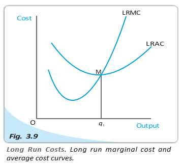
- LRAC shape: The LRAC curve is U-shaped: its falling section reflects IRS, its minimum reflects CRS, and its rising section reflects DRS.
- Minimum point: If LRAC reaches its minimum at output , it falls to the left of and rises to the right.
LRMC and LRAC Relationship
Curve shapes
- LRMC: Like LRAC, it is U-shaped; for the first unit of output, LRMC and LRAC are equal.
- Why MC lies below or above AC: Marginal cost below average cost pulls the average down; marginal cost above average cost pushes it up.
Chapter Summary: Production and Costs
- Production function
- The maximum output possible from given input combinations.
- Short run and long run
- In the short run some inputs are fixed; in the long run all inputs are variable.
- Total, marginal and average product
- Measures of output in relation to the use of a variable input.
- Law of diminishing marginal product
- A production concept describing the change in marginal product as more of a variable input is used.
- Law of variable proportions
- A production concept describing how output changes as a variable input changes while other inputs are fixed.
- Cost function and returns to scale
- Cost function relates output to cost; returns to scale describe output changes when all inputs change.
How do increasing, constant and decreasing returns to scale affect LRAC?
Describe the relationship between LRMC and LRAC.
Quick recap
- All inputs are variable in the long run, so total cost equals total variable cost.
- LRAC is total cost per unit; LRMC is the additional cost of one more unit.
- IRS lowers average cost, CRS keeps it constant, and DRS raises it.
- A typical LRAC curve is U-shaped, with IRS, CRS and DRS corresponding to its falling, minimum and rising sections.
- LRMC crosses LRAC from below at the minimum of LRAC.
- In the short run, the area under SMC up to an output level represents TVC.
Economics — ALL CHAPTERS
1
Introduction
2
Theory of Consumer Behaviour
3
Production And Costs
4
The Theory Of The Firm Under Perfect Competition
5
Market Equilibrium
1
Introduction
2
Collection of Data
3
Organizing of Data
4
Presentation of Data
5
Measures of Central Tendency
6
Correlation
7
Index Numbers
8
Use of Statistical Tools