Class 11 Humanities . Economics . Introductory Micro Economics . Theory of Consumer Behaviour
Chapter 2: Theory of Consumer Behaviour
Ch 2
Economics
Class 11 Humanities
Introduction & Utility
Consumer Choice
- Choice problem: A consumer decides how to spend limited income among goods to obtain the greatest satisfaction.
- What shapes choice: The consumer’s preferences and the prices of goods, together with income, determine which bundle is best.
Bundles and Notation
- Consumption bundle: A combination of quantities of goods chosen by a consumer.
- Two-good example: The chapter simplifies choice by considering bananas and mangoes, denoted by quantities .
- Example: The bundle consists of 5 bananas and 10 mangoes.
Utility
- Utility: The want-satisfying capacity of a commodity; it represents the satisfaction a consumer derives from it.
- Subjective nature: Different people may derive different utility from the same good, and a person’s utility may vary with time and place.
Cardinal Utility and Its Measures
Find the extra satisfaction from the nth unit by subtracting the total utility of the previous quantity.
Example: Marginal Utility
- Given: 4 bananas give units of TU and 5 bananas give units.
- Calculation: units.
Total utility from n units equals the sum of the marginal utilities of those units.
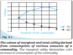
Law of Diminishing Marginal Utility
- Law: With consumption of other goods held constant, marginal utility from each additional unit of a commodity declines as its consumption increases.
- Reason: As a consumer obtains more of a good, the desire for still more of it becomes weaker.
- Effect on total utility: Total utility rises at a diminishing rate while marginal utility is positive; when marginal utility is zero, total utility is at its maximum, and negative marginal utility makes total utility fall.
Demand and the Demand Curve
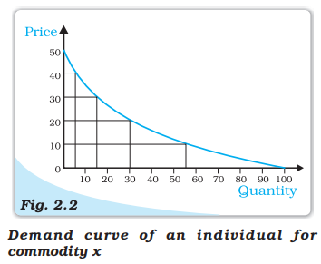
Law of Demand and Its Utility Explanation
Define marginal utility and write its general formula.
State the law of diminishing marginal utility.
How does diminishing marginal utility help explain a downward-sloping demand curve?
Quick recap
- Consumer choice depends on preferences, prices and income; cardinal and ordinal utility are two approaches to explaining it.
- A bundle gives quantities of bananas and mangoes, respectively.
- Utility is subjective and can vary across people, places and times.
- TU is total satisfaction; MU is the change in TU from one additional unit.
- Diminishing MU means successive units generally add less satisfaction; MU may reach zero or become negative.
- Diminishing MU explains why consumers pay less for additional units and why the demand curve slopes downward.
Ordinal Utility Analysis
Ordinal Utility and Indifference Curves
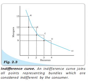
Marginal Rate of Substitution
For bananas and mangoes, this is the absolute change in mangoes divided by the change in bananas along an indifference curve.
Law of Diminishing Marginal Rate of Substitution
| Bundle | Bananas () | Mangoes () | Mangoes sacrificed per extra banana |
|---|---|---|---|
| A | 1 | 15 | — |
| B | 2 | 12 | 3:1 |
| C | 3 | 10 | 2:1 |
| D | 4 | 9 | 1:1 |
Indifference Curves for Perfect Substitutes
| Bundle | Notes () | Coins () | Coins sacrificed per extra note |
|---|---|---|---|
| A | 1 | 8 | — |
| B | 2 | 7 | 1:1 |
| C | 3 | 6 | 1:1 |
| D | 4 | 5 | 1:1 |
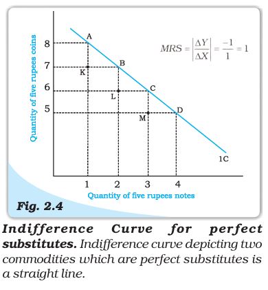
Monotonic Preferences
State the law of diminishing marginal rate of substitution.
How do indifference curves differ for ordinary goods and perfect substitutes?
Quick recap
- Ordinal utility ranks bundles instead of measuring satisfaction numerically.
- An indifference curve joins bundles that provide equal satisfaction.
- MRS measures the amount of one good sacrificed for an extra unit of another while satisfaction stays constant.
- Diminishing MRS makes the usual indifference curve convex to the origin.
- Perfect substitutes have constant MRS and straight-line indifference curves.
- Monotonic preferences favour more of at least one good and no less of the others.
Indifference Map
Indifference Map
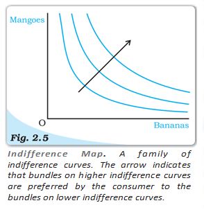
Indifference map — A family of indifference curves showing a consumer’s preferences over different bundles of goods.
- Same curve: Every bundle on one indifference curve gives the consumer the same satisfaction.
- Higher curve: With monotonic preferences, bundles on a higher indifference curve are preferred to bundles on a lower one.
Features of Indifference Curves
- Higher indifference curves: With monotonic preferences, a curve farther from the origin represents bundles that give greater satisfaction.
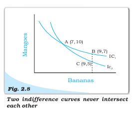
- No intersection: Two indifference curves cannot intersect, because an intersection would imply that distinct bundles provide both equal and unequal satisfaction.
- Convexity: Diminishing marginal rate of substitution generally makes an indifference curve convex to the origin.
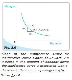
1. Indifference Curves Slope Downwards
- Trade-off: On the same curve, gaining more bananas must be balanced by giving up some mangoes to keep satisfaction unchanged.
- Reason: More bananas with the same mango quantity would move the consumer to a higher curve, not leave them on the same curve.
2. Higher Indifference Curves Give Greater Utility
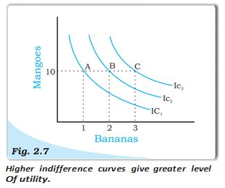
- Positive marginal utility: If having more of a good adds satisfaction, the consumer prefers a bundle with more of that good and the same quantity of the other.
- Higher utility: A bundle with more mangoes, more bananas, or more of both lies on a higher-preference curve than a bundle with less.
| Bundle | Bananas | Mangoes | Preference |
|---|---|---|---|
| A | 1 | 10 | Lowest |
| B | 2 | 10 | Higher than A |
| C | 3 | 10 | Higher than B |
3. Indifference Curves Never Intersect
- Contradiction: If two curves intersect at A, then A is indifferent to a point on each curve; by transitivity, those two points must also be equally preferred.
- Why impossible: The bundles represented on the two curves imply different preference levels under monotonicity, so the intersection gives conflicting rankings.
What does an indifference map show?
Why does an indifference curve slope downwards?
Why can two indifference curves not intersect?
Quick recap
- An indifference map is a family of curves representing a consumer’s preferences.
- Bundles on the same indifference curve give equal satisfaction.
- An indifference curve slopes downward because more of one good requires less of the other to maintain satisfaction.
- With positive marginal utility, a bundle with more of a good is preferred, other things unchanged.
- Higher indifference curves represent greater utility.
- Indifference curves do not intersect because intersection would create inconsistent preference rankings.
The Consumer’s Budget
Budget Set and Budget Constraint
Example: Affordable Bundles
- Given: Income is Rs. 20; both goods cost Rs. 5 per unit and are available only in integral units.
- Exhausting the budget: , , , and each cost exactly Rs. 20.
- Underspending: Other listed affordable bundles, such as or , cost less than Rs. 20.
- Unaffordable: and cost more than Rs. 20.
Budget Line and Its Slope
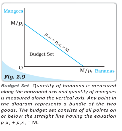
Price ratio and budget-line slope — The absolute slope measures the quantity of mangoes the consumer must give up to obtain one more banana while remaining on the budget line.
Deriving the Slope of the Budget Line
- Take two points on the same budget line: and .
- Both bundles spend the full income.
- Subtract the first budget equation from the second.
- Rearrange to obtain the slope.
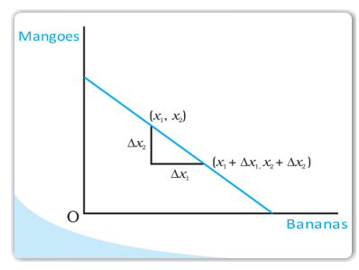
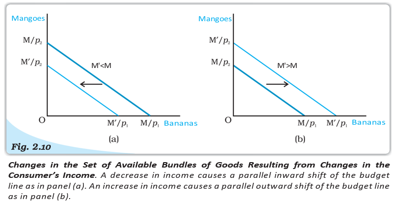
Changes in the Budget Set
| Change | Budget-line effect |
|---|---|
| Income rises: | Both intercepts increase; the line shifts parallel outward. The slope stays . |
| Income falls: | Both intercepts decrease; the line shifts parallel inward. The slope stays . |
Prices remain unchanged; replace income with .
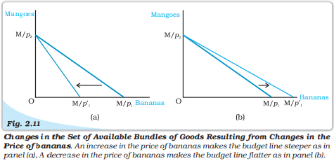
| Change | Budget-line effect |
|---|---|
| Banana price rises: | Vertical intercept stays fixed; horizontal intercept falls. The line pivots inward around the vertical intercept and becomes steeper. |
| Banana price falls: | Vertical intercept stays fixed; horizontal intercept rises. The line pivots outward around the vertical intercept and becomes flatter. |
Income and the mango price remain unchanged.
Change in Mango Price
- Mango price change: If income and the banana price stay fixed, a change in the mango price similarly changes the slope and pivots the budget line around its unchanged horizontal intercept.
What does the absolute slope of the budget line represent?
What happens to the budget line when income rises and prices remain unchanged?
What happens when the price of bananas rises, with income and the mango price unchanged?
Quick recap
- Budget constraint: Affordable bundles satisfy .
- Budget line: Bundles that use all income satisfy .
- Intercepts: The banana and mango intercepts are and , respectively.
- Slope: The budget-line slope is ; its absolute value is the goods’ price ratio.
- Income change: With prices fixed, income changes shift the budget line in parallel.
- Price change: Changing one good’s price pivots the line around the intercept for the good whose price is unchanged.
Optimal Choice Of The Consumer
Consumer Preferences and Rational Choice
- Preferences: Consumers are assumed to have well-defined preferences and to be able to compare any two bundles, either preferring one or being indifferent between them.
- Rational choice: A rational consumer chooses the most preferred bundle from those available in the budget set.
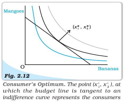
Location of the Consumer’s Optimum
At an interior optimum, the absolute slope of the indifference curve (the MRS) equals the absolute slope of the budget line (the price ratio).
| Rate | Meaning |
|---|---|
| MRS | How much of one good the consumer is willing to give up for another. |
| Price ratio | How much of one good the market requires the consumer to give up for another. |
| At the optimum | The willingness to substitute equals the market’s substitution rate. |
Why Tangency Matters
- If MRS exceeds the price ratio: The consumer is willing to give up more of one good than the market requires to obtain the other, so she can move to a preferred bundle.
- Example: If mangoes and bananas have equal prices, the price ratio is . If the consumer’s MRS is , she is willing to give up two mangoes for a banana, while the market requires only one.
- If MRS is below the price ratio: A similar adjustment can improve the consumer’s bundle.
- Therefore: Equality of MRS and the price ratio is the condition for an interior optimum.
Demand
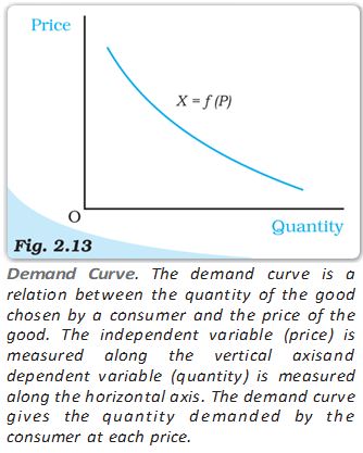
- Demand: The quantity of a good a consumer is willing and able to buy, given prices, income, and preferences.
- Determinants: A consumer’s choice depends on the good’s own price, prices of related goods, income, and tastes and preferences.
Demand Function and Law of Demand
is quantity demanded and is the good’s price; other determinants are held constant.
Functions and Their Graphs
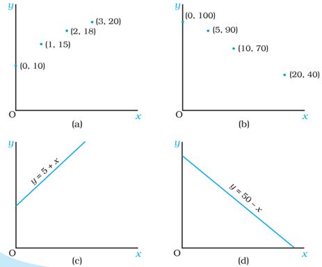
Reading Function Graphs
- Usual convention: The independent variable is on the horizontal axis and the dependent variable on the vertical axis.
- Economics convention: The demand curve commonly places price on the vertical axis and quantity demanded on the horizontal axis.
- Slope: An increasing function slopes upward; a decreasing function slopes downward.
- Budget set
- All bundles available to the consumer at given resources and prices.
- Monotonic preferences
- Preferences under which more of at least one good and no less of the others is preferred.
- MRS
- The rate at which the consumer is willing to substitute one good for another.
- Demand
- The quantity of a good the consumer is willing and able to buy.
- Demand curve
- A graphical representation of the demand function.
Where is the consumer’s optimum located?
State the tangency condition for an interior optimum.
State the law of demand.
Quick recap
- A rational consumer chooses the most-preferred bundle in the budget set.
- With monotonic preferences, the optimum lies on the budget line.
- At an interior optimum, the MRS equals the price ratio.
- Demand is the quantity a consumer is willing and able to buy at given conditions.
- A demand function gives optimal quantity as a function of price, holding other factors constant.
- Demand generally falls as price rises; the demand curve slopes downward.
Deriving ADemand Curve From Indifference Curves And Budget Constraints
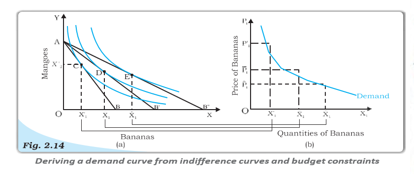
Deriving a Demand Curve
Demand curve — A demand curve shows the quantities a consumer chooses at different prices, with income and other relevant factors held constant.
From consumer equilibrium to demand
- Starting point: With income and prices of bananas and mangoes fixed, the consumer chooses an equilibrium bundle on the highest affordable indifference curve.
- Price falls: If the price of bananas falls while income and the price of mangoes stay constant, the budget set expands and the consumer reaches a higher indifference curve.
- Quantity response: The consumer buys more bananas at the lower price; repeating this for further price falls gives additional price–quantity points.
- Demand curve: Plot each banana price against the quantity chosen at that price. The resulting curve slopes downward.
Why the Demand Curve Slopes Downward
| Effect | How it works | Impact on demand for bananas |
|---|---|---|
| Substitution effect | Bananas become cheaper relative to mangoes, so the consumer substitutes bananas for mangoes. | Raises banana demand. |
| Income effect | The price fall increases the consumer’s purchasing power. | Raises demand for bananas if they are a normal good. |
Law of Demand — Other things being equal, price and quantity demanded are negatively related: a price rise lowers demand, while a price fall raises it.
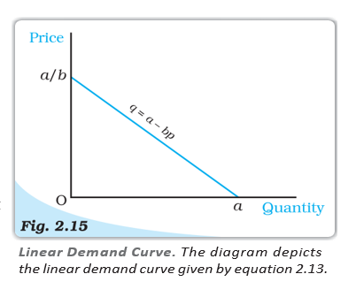
Linear Demand
is quantity demanded at price ; is the vertical intercept and is the slope.
Reading the equation
- Quantity intercept: At price , demand is .
- Price intercept: At price , demand is zero.
- Slope: For each one-unit increase in price, demand falls by units.
Normal, Inferior and Giffen Goods
Demand function — A demand function relates the quantity demanded of a good to its price, with other factors held constant.
| Point | Normal good | Inferior good |
|---|---|---|
| As income rises | Demand rises. | Demand falls. |
| As income falls | Demand falls. | Demand rises. |
| Income–demand relation | Same direction. | Opposite directions. |
| Example | Most goods. | Low-quality foods such as coarse cereals. |
A Good Can Change Category
- Income levels matter: A good may be normal at one income level and inferior at another.
- Example: At very low incomes, rising income may increase demand for coarse cereals; beyond a point, higher income may lead consumers to switch to better-quality cereals.
Giffen good — An inferior good for which demand rises when its price rises because the income effect outweighs the opposing substitution effect.
How a Giffen Response Can Occur
- Price rises → purchasing power falls.
- For an inferior good, the income effect can increase its demand.
- If this income effect is stronger than the substitution effect, quantity demanded rises with price.
Substitutes and Complements
| Point | Complementary goods | Substitute goods |
|---|---|---|
| Meaning | Goods consumed together. | Goods that can replace each other. |
| Examples | Tea and sugar; shoes and socks; pen and ink. | Tea and coffee. |
| Effect of a related good’s price rise | Demand for the good falls; their prices and demands move in opposite directions. | Demand for the good rises as consumers switch to it; they move in the same direction. |
How do indifference curves and budget constraints help derive a demand curve?
What makes a good Giffen?
Quick recap
- Changing a good’s price while holding other factors constant reveals the consumer’s price–quantity choices.
- For ordinary goods, price falls raise demand through substitution and income effects.
- The law of demand states that price and quantity demanded are negatively related, other things equal.
- A linear demand function has intercepts and , with slope .
- Normal-good demand moves with income; inferior-good demand moves against income.
- A Giffen good is an inferior good whose demand rises with price when the income effect dominates.
- Demand moves opposite to the price of a complement and in the same direction as the price of a substitute.
Shifts In The Demand Curve
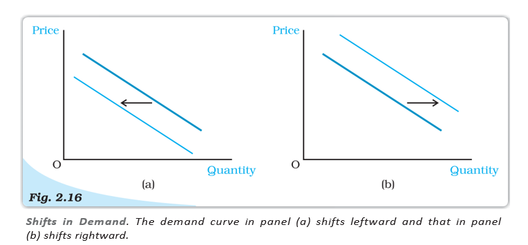
Shifts in the Demand Curve
Examples of preference shifts
- Ice-creams: Greater preference in summer can shift demand rightward.
- Cold drinks: Information that they may harm health can reduce preference and shift demand leftward.
Movements Along the Curve vs Shifts
Demand function — A relation between the quantity demanded and the good’s price, with other factors held constant.
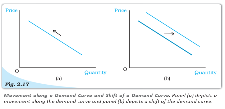
- Own-price change: A higher price generally means lower quantity demanded, and a lower price means higher quantity demanded; this is movement along the curve.
- Other-factor change: Changes in income, related-good prices, or preferences shift the curve.
- Demand curve: A graph of the demand function.
Market Demand
Add individual quantities demanded at the same price.
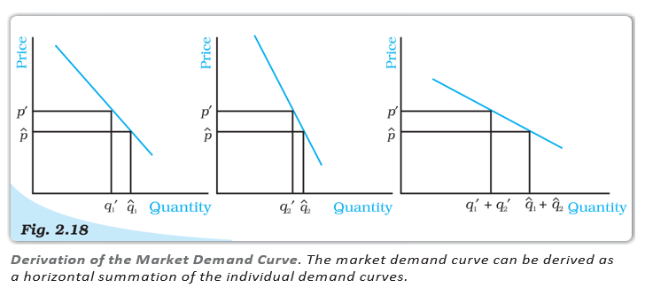
Adding Two Linear Demand Curves
The first consumer demands zero above ; both demand zero above .
How does a rise in the price of a complement affect demand for a good?
What is horizontal summation of demand curves?
Quick recap
- A change in a factor other than the good’s own price shifts its demand curve.
- Normal-good demand rises with income; inferior-good demand falls with income.
- A higher substitute price shifts demand right; a higher complement price shifts it left.
- Own-price changes cause movement along the demand curve; other-factor changes shift it.
- Market demand is the sum of all consumers’ quantities demanded at each price.
- Horizontal summation of the example curves gives up to , then up to , and zero above.
Elasticity Of Demand
Meaning and Measurement of Price Elasticity
Price elasticity of demand — A measure of how responsive quantity demanded is to a change in the good’s price.
Key points
- Responsiveness: Demand may change considerably or very little in response to a price change.
- Sign: Price and demand usually move in opposite directions, so signed elasticity is negative.
- Convention: For simplicity, elasticity categories use the absolute value, .
Divide the percentage change in quantity demanded by the percentage change in price. For finite changes, use the initial quantity and price as the percentage bases.
| Measure | Calculation | Percentage change |
|---|---|---|
| Quantity demanded | ||
| Price | ||
| Price elasticity | (inelastic) |
Elastic, Inelastic and Unitary-Elastic Demand
| Type | Comparison of percentage changes | Absolute elasticity | Typical example |
|---|---|---|---|
| Inelastic | Quantity demanded changes by less than price | Essential goods | |
| Elastic | Quantity demanded changes by more than price | Luxury goods | |
| Unitary elastic | Quantity demanded changes by the same percentage as price | Equal percentage responses |
Elasticity can vary with price
- At different prices: The same good may be elastic, unitary elastic or inelastic at different points on its demand curve.
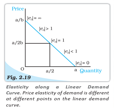
Elasticity Along a Linear Demand Curve
Formula and variation
- Linear demand curve: Let , where . Its slope is constant: .
- Elasticity at a point: Substitution into the elasticity formula gives signed elasticity .
- Variation: Elasticity differs at different points on the same straight-line demand curve.
| Position | Condition | Absolute elasticity |
|---|---|---|
| Horizontal-axis intercept | ||
| Between the horizontal-axis intercept and midpoint | ||
| Midpoint | ||
| Between midpoint and vertical-axis intercept | ||
| Vertical-axis intercept |
Geometric Measure on a Straight-Line Demand Curve
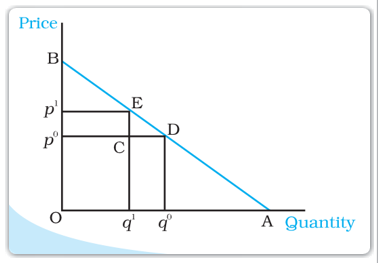
Segment-ratio method
- Rule: At any point on a straight-line demand curve, elasticity equals the lower segment divided by the upper segment.
- Formula: , where is the lower segment and the upper segment, as labelled on the curve.
- Along the curve: Elasticity is greater than one to the left of the midpoint, one at the midpoint, and less than one to the right.
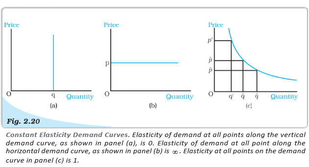
Constant-Elasticity Demand Curves
| Curve | Demand response | Absolute elasticity | Classification |
|---|---|---|---|
| Vertical | Quantity remains fixed at every price | Perfectly inelastic | |
| Horizontal | At the stated market price, quantity may vary; at another price, quantity demanded drops to zero | Perfectly elastic | |
| Rectangular hyperbola | Equal percentage changes in price and quantity along the curve | Unitary elastic |
- Price elasticity of demand
- Responsiveness of quantity demanded to a price change.
- Inelastic demand
- Demand changes by a smaller percentage than price.
- Elastic demand
- Demand changes by a larger percentage than price.
- Unitary-elastic demand
- Demand and price change by equal percentages.
- Perfectly inelastic demand
- Quantity demanded does not respond to price.
- Perfectly elastic demand
- Elasticity is infinite at the stated market price.
How is price elasticity of demand calculated?
How does elasticity vary along a linear demand curve?
Quick recap
- Price elasticity measures responsiveness of quantity demanded to a price change.
- Use percentage changes; demand and price usually move in opposite directions, making signed elasticity negative.
- Classify demand using absolute elasticity: below one is inelastic, equal to one is unitary elastic, and above one is elastic.
- For a linear curve , elasticity varies from zero to infinity and equals one at the midpoint.
- On a straight-line curve, geometric elasticity is the lower segment divided by the upper segment.
- Vertical, horizontal and rectangular-hyperbola demand curves have elasticities of zero, infinity and one, respectively.
Factors Determining Price Elasticity of Demand for a Good
Factors Determining Price Elasticity of Demand
Nature of the Good and Availability of Substitutes
- Necessities: Demand usually responds little to price changes, so necessities such as food tend to have price-inelastic demand.
- Luxuries: Demand is generally more responsive to price changes, so luxury goods tend to have price-elastic demand.
- Close substitutes: A good is more likely to have elastic demand when consumers can readily switch to close substitutes.
- Specific varieties: Demand for a particular variety of pulses may be elastic because consumers can switch to another variety, even when demand for food overall is inelastic.
- Few substitutes: When close substitutes are not readily available, demand is likely to be inelastic.
Elasticity and Expenditure
Total expenditure — Total expenditure on a good equals its price multiplied by the quantity demanded.
Use this to calculate expenditure at a given price and quantity.
Price Change, Elasticity and Expenditure
- Price and demand: Price and quantity demanded generally move in opposite directions; the effect on expenditure depends on how strongly demand responds.
- Price rises: If quantity falls by a greater percentage than price rises, expenditure falls; if it falls by a smaller percentage, expenditure rises.
- Price falls: If quantity rises by a greater percentage than price falls, expenditure rises; if it rises by a smaller percentage, expenditure falls.
- Equal percentage changes: Expenditure remains unchanged when the percentage change in quantity equals the percentage change in price.
| Case | Price change | Quantity change | Expenditure | Demand type |
|---|---|---|---|---|
| 1 | Rises by 10% | Falls by 8% | Rises | Inelastic |
| 2 | Rises by 10% | Falls by 12% | Falls | Elastic |
| 3 | Rises by 10% | Falls by 10% | Unchanged | Unit elastic |
| 4 | Falls by 10% | Rises by 15% | Rises | Elastic |
| 5 | Falls by 10% | Rises by 7% | Falls | Inelastic |
| 6 | Falls by 10% | Rises by 10% | Unchanged | Unit elastic |
| Demand type | Quantity response compared with price change | Expenditure response |
|---|---|---|
| Elastic | Greater percentage change | Moves opposite to price |
| Inelastic | Smaller percentage change | Moves in the same direction as price |
| Unit elastic | Equal percentage change | Remains unchanged |
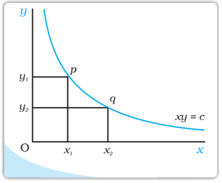
Rectangular Hyperbola
Rectangular hyperbola — A downward-sloping curve represented by , where is constant.
Constant Expenditure on a Rectangular-Hyperbola Demand Curve
- Demand curve: If price and quantity satisfy , where is constant, the demand curve is a rectangular hyperbola.
- Expenditure: At every point on this curve, price multiplied by quantity equals ; total expenditure is therefore constant.
- Equal areas: The rectangles formed by the axes and any two points on the curve have the same area.
Relationship Between Elasticity and Change in Expenditure
Approximate Change in Expenditure
- Initial expenditure: At price and quantity , expenditure is .
- After a change: At price and quantity , expenditure is .
- Exact change: Expanding the new expenditure and subtracting the initial expenditure gives .
- Small changes: When and are small, the product term is negligible, so .
- Signed elasticity: Price elasticity of demand is a pure number; in the signed convention, and is generally negative.
For small changes in price and quantity, using signed price elasticity.
| Signed elasticity | Demand type | Expenditure compared with price |
|---|---|---|
| Elastic | Changes in the opposite direction | |
| Inelastic | Changes in the same direction | |
| Unit elastic | Remains unchanged |
How does price elasticity determine the effect of a price rise on total expenditure?
Why does a rectangular-hyperbola demand curve imply constant expenditure?
Quick recap
- Necessities and goods with few close substitutes tend to have inelastic demand; luxuries and goods with close substitutes tend to have elastic demand.
- Total expenditure is price multiplied by quantity demanded: .
- With elastic demand, expenditure moves opposite to price; with inelastic demand, it moves in the same direction.
- With unit-elastic demand, expenditure remains unchanged.
- A rectangular-hyperbola demand curve, , gives constant expenditure.
- Price elasticity of demand is a pure number; with signed elasticity, for small changes.
Economics — ALL CHAPTERS
1
Introduction
2
Theory of Consumer Behaviour
3
Production And Costs
4
The Theory Of The Firm Under Perfect Competition
5
Market Equilibrium
1
Introduction
2
Collection of Data
3
Organizing of Data
4
Presentation of Data
5
Measures of Central Tendency
6
Correlation
7
Index Numbers
8
Use of Statistical Tools