Class 11 Humanities . Economics . Statistics For Economics . Measures of Central Tendency
Chapter 5: Measures of Central Tendency
Ch 5
Economics
Class 11 Humanities
Introduction
Why Summarise Data?
Purpose of an average
- Large data sets can be difficult to understand or compare when every value is considered separately.
- A single representative value gives a brief summary of the data and helps draw meaningful conclusions.
- Everyday examples include average marks, rainfall, factory production and income.
Measures of Central Tendency
Measure of central tendency — A statistical measure that summarises a data set with one typical or representative value.
Common averages
- Arithmetic Mean indicates the ordinary average.
- Median identifies the middle value, dividing the observations so that half lie on either side.
- Mode identifies the value that occurs most often.
- Geometric Mean and Harmonic Mean are other averages used in certain situations; this lecture focuses on the first three.
Choosing a Representative Value
| Measure | Question it answers |
|---|---|
| Arithmetic Mean | Is Baiju’s landholding above the ordinary average? |
| Median | Is Baiju’s landholding greater than the land owned by half the farmers? |
| Mode | Is Baiju’s landholding greater than the size most farmers own? |
Example: Balapur farmers
- Context: Baiju is a farmer with 1 acre of land in Balapur, a village in Buxar district, Bihar, with 50 small farmers.
- Comparison: To assess his relative economic condition, compare his landholding with the village’s landholding data using an appropriate average.
- Choice matters: The mean, median and mode answer different questions, so the useful average depends on what is being compared.
- Central tendency
- The tendency of data values to cluster around a representative centre.
- Average
- A statistical value used to represent or summarise a data set.
- Arithmetic Mean
- The ordinary average of a set of values.
- Median and Mode
- The median is the middle value; the mode is the most frequently occurring value.
What is a measure of central tendency?
Quick recap
- Central tendency summarises a data set using one representative value.
- Averages help make large sets of data easier to understand and compare.
- The three main averages in this lecture are the arithmetic mean, median and mode.
- Mean gives the ordinary average; median marks the middle; mode is the most frequent value.
- Choose the average that best answers the question being asked.
- Geometric mean and harmonic mean are other averages used in particular situations.
Arithmetic Mean
Meaning and General Formula
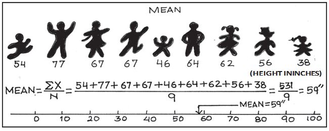
Arithmetic mean — The arithmetic mean is the sum of all observations divided by the number of observations; it is the most commonly used measure of central tendency.
- Notation: The arithmetic mean is usually denoted by .
- Interpretation: It represents the average value of the observations.
Here, is an observation and is the total number of observations.
Example: Family incomes
- Data: Six monthly incomes are Rs. 1,600, Rs. 1,500, Rs. 1,400, Rs. 1,525, Rs. 1,625 and Rs. 1,630.
- Mean: The total is Rs. 9,280; dividing by gives approximately Rs. 1,546.67, or about Rs. 1,547.
Methods of Calculation
| Form | What is given |
|---|---|
| Ungrouped data | Individual observations |
| Grouped data | Values with frequencies, or class intervals with frequencies |
Ungrouped Data: Direct Method
- Rule: Add all observations and divide by their count.
- Use: Apply this method when the observations can be added conveniently.
Example: Test marks
- Data: Marks are ; their total is .
- Mean: marks.
Ungrouped Data: Assumed Mean Method
Assumed mean — A convenient reference value chosen temporarily to simplify calculations of the arithmetic mean.
- When useful: Use this method when there are many observations or the figures are large.
- Choice: Any value, whether in the data or not, can be used; a central value usually makes calculations easier.
- Deviation: For each observation, calculate , where is the assumed mean.
Add the average deviation to the assumed mean.
Example: Weekly family incomes
- Data: Ten weekly incomes total Rs. 11,160; take .
- Deviation total: .
- Mean: .
Ungrouped Data: Step-Deviation Method
- Purpose: Reduce large deviations by dividing each deviation by a common factor .
- Scaled deviation: Calculate , then use the step-deviation formula.
Here, is the assumed mean, is the common factor and is the number of observations.
Weekly income example by step deviation
- Values: With and , the scaled deviations total .
- Mean: .
Grouped Data: Discrete Series
- Discrete series: Each distinct value is listed with its frequency .
- Direct method: Multiply each value by its frequency, add the products, then divide by the total frequency.
is the total of frequency–value products; is the total frequency.
Example: Housing plots
- Data: Plot sizes are square metres, with frequencies .
- Totals: and .
- Mean: The average plot size is square metres.
Assumed mean and step deviation for a discrete series
- Assumed mean: Multiply each deviation by its frequency; use .
- Step deviation: Use , multiply by frequency, and apply .
Grouped Data: Continuous Series
- Continuous series: Data are arranged in class intervals, each with a frequency.
- Midpoint: Use each class interval's midpoint as its representative value.
- Interval types: Intervals may be exclusive, inclusive or unequal; calculate the mean in the same way for all three types.
Find each midpoint, then treat the midpoints as the values of a discrete series.
| Class interval | Frequency | Midpoint | |
|---|---|---|---|
| – | 5 | 5 | 25 |
| – | 12 | 15 | 180 |
| – | 15 | 25 | 375 |
| – | 25 | 35 | 875 |
| – | 8 | 45 | 360 |
| – | 3 | 55 | 165 |
| – | 2 | 65 | 130 |
| Total | 70 | 2,110 |
Continuous-series calculation
- Direct method: marks.
- Step deviation: Taking and , ; therefore marks.
Properties of the Arithmetic Mean
- Zero-deviation property: The sum of deviations from the arithmetic mean is always zero.
- Effect of extremes: Very large or very small values can pull the mean towards them.
The deviations of all observations from their arithmetic mean cancel out.
Do not assume the mean is unaffected by extreme values; a very large or small observation can shift it.
Weighted Arithmetic Mean
Weighted arithmetic mean — An average that gives different importance to observations by assigning each a weight.
- Why use it: A price change in a more important commodity may deserve greater influence on the average.
- Example: A consumer's budget shares for mangoes and potatoes can be used as their weights.
is the weight assigned to value .
- Observation
- An individual value in a data set.
- Frequency
- The number of times a value or class occurs.
- Assumed mean
- A convenient reference value used to simplify mean calculations.
- Weight
- A number representing the relative importance assigned to an observation.
How is the arithmetic mean calculated for a continuous series?
State two properties of the arithmetic mean.
Quick recap
- Arithmetic mean, the most commonly used measure of central tendency, equals the sum of observations divided by their count.
- For ungrouped data, use the direct, assumed mean or step-deviation method.
- For a discrete series, multiply each value by its frequency before averaging.
- For a continuous series, use class midpoints as the representative values.
- Deviations from the mean sum to zero, but extreme values can shift it.
- A weighted mean reflects the relative importance of observations.
Median
Meaning and Properties
Median for Individual Observations
Finding the Median
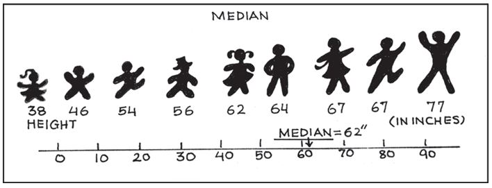
- First: Arrange observations in ascending or descending order.
- Odd number of observations: The middle observation is the median. For , the median is .
- Even number of observations: Take the arithmetic mean of the two middle values. For 20 students' marks, the middle values are and , so the median is marks.
This gives the position in the ordered array, not the median value itself.
Median for a Discrete Series
Using Cumulative Frequency
- Locate the position: Find the th item, where is the total frequency.
- Use cumulative frequency: Find the first cumulative frequency that includes this position; its corresponding variable value is the median.
| Income (Rs.) | Frequency () | Cumulative frequency () |
|---|---|---|
| 10 | 2 | 2 |
| 20 | 4 | 6 |
| 30 | 10 | 16 |
| 40 | 4 | 20 |
Example: Median Income
- Total frequency: , so the median position is th item.
- Locate the item: The th item falls within cumulative frequency , corresponding to income Rs. 30.
- Median income: Rs. 30.
Median for a Continuous Series
Median class — The class interval containing the th item.
Use the cumulative frequency of the class preceding the median class. No adjustment is required when frequencies are of unequal size or magnitude.
Symbols and Example: Daily Wages
- Symbols: = lower limit of the median class; = cumulative frequency before it; = its frequency; = class-interval width.
- Find the position: Total workers , so . The th item lies in the – wage class.
- Substitute: .
- Interpretation: About half the workers earn less than or equal to Rs. 35.83 and half earn more than or equal to this amount.
| Daily wages (Rs.) | Workers () | Cumulative frequency |
|---|---|---|
| – | 14 | 14 |
| – | 28 | 42 |
| – | 33 | 75 |
| – | 30 | 105 |
| – | 20 | 125 |
| – | 15 | 140 |
| – | 13 | 153 |
| – | 7 | 160 |
Do not confuse the median's position with its value: the position formula identifies the item; the corresponding observation or class formula gives the median.
Quick recap
- Order the data before locating its middle.
- For an even number of observations, average the two middle values.
- For a discrete series, locate the th item using cumulative frequency.
- For a continuous series, locate the th item and identify its median class.
- Use for the continuous-series median; no adjustment is needed for unequal frequencies.
- The median is positional and is less affected by extreme values.
Quartiles
Quartiles
Percentiles
Percentile example
- Out of 100,000 candidates: About 82,000 are below an 82nd-percentile candidate and 18,000 are above.
Calculating Quartiles
Arrange the observations in ascending order first. is the number of observations.
Example: lower quartile
- Ordered marks: ; hence .
- Position: is at the th item.
- Interpolate: marks.
Mode
- Purpose: Mode identifies the most typical or frequently occurring value in a distribution.
- Use: It is useful for finding the most popular product choice, such as the most demanded shoe size or shirt style.
- Notation: Mode is denoted by ; a distribution may have one mode, more than one mode, or no mode.
Mode in a Discrete Series
| Type | Meaning | Example |
|---|---|---|
| Unimodal | One value has the highest frequency. | Values with frequencies : mode is . |
| Bimodal | Two values share the highest frequency. | Two values occur most often. |
| Multimodal | More than two values share the highest frequency. | Several values occur equally often and most often. |
| No mode | No value occurs more often than the others. |
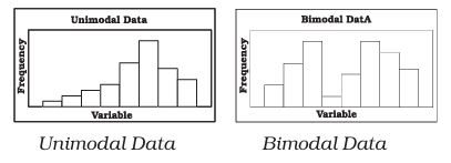
Mode in a Continuous Series
Modal class — The class interval with the largest frequency in a continuous frequency distribution.
is the lower limit of the modal class; and are the absolute differences between its frequency and the frequencies of the preceding and succeeding classes, respectively. is the class interval.
Conditions for using the grouped-data formula
- Class intervals: They should be equal and the series should be exclusive.
- Given midpoints: Work out the class intervals before identifying the modal class.
Finding mode from a cumulative frequency distribution
- Convert cumulative frequencies into ordinary frequencies by taking successive differences.
- Identify the class with the largest frequency as the modal class.
- Find , , and from that class and its neighbouring classes.
- Substitute these values into the grouped-data mode formula.
| Income group | Frequency |
|---|---|
| – | |
| – | |
| – | |
| – | |
| – | |
| – | |
| – | |
| – |
Grouped mode example
- Modal class: –, with frequency .
- Values: , , , and .
- Substitution: thousand rupees, or about Rs. 27,727.
Check the arithmetic after substituting into the mode formula: , not .
Which average is most suitable for finding the shoe size with the greatest demand?
Quick recap
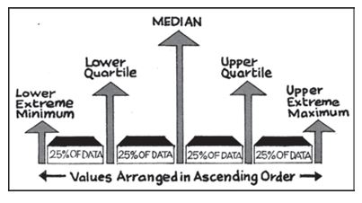
- , and divide ordered data into four equal parts; the central 50% lies between and .
- Percentiles divide a distribution into 100 parts; is the median.
- For an individual or discrete series, quartile positions are and .
- Mode is the most frequent value; a distribution can be unimodal, bimodal, multimodal or have no mode.
- For grouped continuous data, identify the modal class and apply .
- Convert cumulative frequencies to ordinary frequencies using successive differences before finding grouped mode.
Relative Position Of Arithmetic Mean, Median And Mode
Relative Position of the Three Averages
- Notation: Arithmetic mean = , median = , and mode = .
- Possible orders: or .
- Relationship: The median lies between the arithmetic mean and the mode.
Choosing an Appropriate Average
| Measure | Meaning | Features and limitations |
|---|---|---|
| Arithmetic mean | Sum of all observations divided by the number of observations. | Common and simple to calculate; uses all observations, but is strongly affected by extreme values. |
| Median | The central value, with equal numbers of observations below and above it. | A better summary when extreme values affect the mean; can be found graphically and used for open-ended distributions. |
| Mode | The value occurring most frequently. | Useful for describing qualitative data; can be found graphically and used for open-ended distributions. |
Other Key Properties
- Mean deviations: The sum of deviations of all observations from their arithmetic mean is zero.
- Weights: Weights may be assigned to observations according to their importance.
- Quartiles: They divide the total set of values into four equal parts.
- Selection: Choose an average according to the purpose of analysis and the nature of the distribution.
Quick recap
- Central tendency summarises a data set with one representative value.
- The arithmetic mean is the sum of observations divided by their number; it uses all values but is affected by extremes.
- The sum of deviations of observations from their arithmetic mean is zero.
- Weights may be assigned to observations according to their importance.
- The median is central, and the mode is the most frequent value.
- The median lies between the mean and mode: or .
- Quartiles divide values into four equal parts; select an average to suit the data and analysis.
Economics — ALL CHAPTERS
1
Introduction
2
Theory of Consumer Behaviour
3
Production And Costs
4
The Theory Of The Firm Under Perfect Competition
5
Market Equilibrium
1
Introduction
2
Collection of Data
3
Organizing of Data
4
Presentation of Data
5
Measures of Central Tendency
6
Correlation
7
Index Numbers
8
Use of Statistical Tools