Class 11 Humanities . Economics . Statistics For Economics . Organizing of Data
Chapter 3: Organizing of Data
Ch 3
Economics
Class 11 Humanities
Introduction
Classification of Data
Classification — Arranging or organising things into groups or classes based on some criterion.
- Purpose: Classification brings order to raw data and makes further statistical analysis easier.
- Relevant grouping: The criterion should suit the purpose; including unrelated items defeats the purpose of grouping.
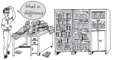
- Benefits: Organised data are easier to locate, compare and use to draw conclusions.
- Example: A junk dealer groups goods as newspapers, plastics, glass and metals, and may sort metals into iron, copper, aluminium and brass.
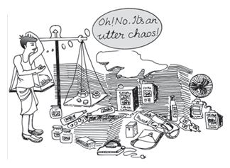
Raw Data and the Need for Organisation
Raw data — Collected data that have not yet been organised or classified.
- Nature: Raw data consist of observations on one or more variables and may be large and cumbersome to handle.
- Difficulty: Finding information or drawing conclusions from large, unclassified data is tedious.
- Next step: After collecting data, organise and present them in classified form before systematic statistical analysis.
- Examples: Marks in mathematics for 100 students and monthly food expenditure for 50 households are raw data when presented without arrangement.
- Census example: India conducts a population census every ten years. In Census 2001, about 20 crore persons were contacted; classifying data by gender, education, marital status and occupation helps reveal the population's structure and nature.
Choosing How to Classify
- Purpose matters: The way data are classified depends on the purpose of the investigation.
- Example: A mathematics teacher may want to know how students performed and how many did not pass.
- Chosen approach: To study the marks in depth, the teacher may construct a frequency distribution; its construction is discussed in the next section.
What is classification of data, and why is it useful?
Why is raw data difficult to analyse?
What determines how data should be classified?
Quick recap
- Classification groups things or data using a relevant criterion.
- Classification brings order to raw data and supports further statistical analysis.
- Raw data are unorganised observations on variables and can be difficult to handle when large.
- Classified data are easier to locate, compare and use to draw conclusions.
- The purpose of an investigation determines the appropriate way to classify data.
- A teacher studying students' marks may construct a frequency distribution.
Classification Of Data
Classification of data — Arranging raw data into groups or classes according to a chosen purpose or characteristic.
Chronological Classification
Chronological classification — Arranging data in ascending or descending order according to time, such as years, quarters, months or weeks.
Example: Population of India
- Time series: Population is a time series when its values are recorded for different years.
- Reading the data: Population rose from 35.7 crores in 1951 to 121.0 crores in 2011.
| Year | Population (crores) |
|---|---|
| 1951 | 35.7 |
| 1961 | 43.8 |
| 1971 | 54.6 |
| 1981 | 68.4 |
| 1991 | 81.8 |
| 2001 | 102.7 |
| 2011 | 121.0 |
Spatial Classification
Spatial classification — Arranging data according to geographical locations, such as countries, states, cities or districts.
| Country | Yield (kg/hectare) |
|---|---|
| Canada | 3594 |
| China | 5055 |
| France | 7254 |
| Germany | 7998 |
| India | 3154 |
| Pakistan | 2787 |
Qualitative Classification
Qualitative classification — Grouping data according to attributes or qualities that cannot be measured numerically.
Attributes
- Examples: Nationality, literacy, religion, gender and marital status.
- Basis for grouping: An attribute is classified by whether a characteristic is present or absent.
- More than one attribute: A population may first be grouped by gender, then each group by married or unmarried status.
Quantitative Classification
Quantitative classification — Grouping data into classes according to characteristics that can be expressed numerically.
Quantitative Characteristics
- Examples: Height, weight, age, income and students’ marks.
- Frequency distribution: A table that shows how many observations fall in each class.
| Marks | Frequency |
|---|---|
| 0–10 | 1 |
| 10–20 | 8 |
| 20–30 | 6 |
| 30–40 | 7 |
| 40–50 | 21 |
| 50–60 | 23 |
| 60–70 | 19 |
| 70–80 | 6 |
| 80–90 | 5 |
| 90–100 | 4 |
| Total | 100 |
Relative frequency — A class frequency expressed as a proportion or percentage of the total frequency.
Here, is the class frequency and is the total frequency.
Reading the Marks Distribution
- Maximum concentration: The 50–60 class has frequency 23, or 23% of the students.
- Minimum concentration: The 0–10 class has frequency 1, or 1% of the students.
Do not confuse qualitative and quantitative classification: grouping objects as living or non-living uses a quality, so it is qualitative.
What is the difference between chronological and spatial classification?
Quick recap
- Classification arranges raw data into groups according to a chosen purpose.
- Chronological classification groups observations by time; data across years can form a time series.
- Spatial classification groups data by place, such as country or state.
- Qualitative classification uses non-measurable attributes; quantitative classification uses measurable characteristics.
- A frequency distribution records the number of observations in each quantitative class.
- Relative frequency is a class frequency expressed as a proportion or percentage of the total.
Variables: Continuous And Discrete
Continuous and Discrete Variables
Continuous variable — A variable that can take any numerical value within a range, including whole, fractional and irrational values.
Discrete variable — A variable that takes only specific, separate values and changes in finite jumps, without taking intermediate values.
| Point | Continuous | Discrete |
|---|---|---|
| Values | Can take any value in a range, including fractional values. | Can take only distinct values; intermediate values are excluded. |
| Change | Varies through infinitely many gradations. | Changes by finite jumps. |
| Examples | Height, weight, time and distance. | Number of students in a class; a variable taking only , , , ... |
Examples and Classification
- Height: A student's height can take values such as cm, cm or cm within a range.
- Student count: A class can have or students, but not .
- Fractions do not determine the type: A variable taking , , , ... is discrete if it cannot take values between successive listed values.
- Continuous examples: Area, volume, temperature, crop yield, rainfall and age.
- Discrete examples: Number appearing on a die, population and number of cars on a road.
Frequency Distribution and Its Terms
Frequency distribution — A systematic classification of quantitative raw data into classes, showing the number of observations in each class.
Classes and Class Frequency
- Class: A range into which observations are grouped; for example, marks may be grouped into –, –, ..., –.
- Class frequency: The number of observations in a particular class.
- Example: The – class has marks in the example, so its frequency is .
- Endpoint note: The raw data also contain two marks of , which are not included in the stated – frequency. The reason for this is left for explanation later in the chapter.
Class limits — The two endpoints of a class: the lower class limit is the lower endpoint and the upper class limit is the upper endpoint.
Class interval (class width) — The difference between a class's upper and lower limits.
For the class –, the class interval is .
Class midpoint (class mark) — The value halfway between a class's lower and upper limits; it represents the class in calculations using grouped data.
For the class –, the class midpoint is .
| Class | Frequency | Lower limit | Upper limit | Class mark |
|---|---|---|---|---|
| – | 1 | 0 | 10 | 5 |
| – | 8 | 10 | 20 | 15 |
| – | 6 | 20 | 30 | 25 |
| – | 7 | 30 | 40 | 35 |
| – | 21 | 40 | 50 | 45 |
| – | 23 | 50 | 60 | 55 |
| – | 19 | 60 | 70 | 65 |
| – | 6 | 70 | 80 | 75 |
| – | 5 | 80 | 90 | 85 |
| – | 4 | 90 | 100 | 95 |
Using Grouped Data
- Grouped observations: Once raw data are arranged into classes, individual observations are generally replaced by their class marks in further calculations.
Frequency Curve
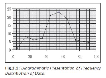
Frequency curve — A graphical representation of a frequency distribution, made by plotting class marks against their frequencies.
Axes
- X-axis: Class marks.
- Y-axis: Class frequencies.
Why is the number of students in a class a discrete variable?
How is a class midpoint found, and what does it represent?
Quick recap
- Continuous variables can take any value within a range; discrete variables take separate values without intermediate values.
- A discrete variable may take fractional values if only specific fractions are allowed.
- A frequency distribution groups quantitative data into classes and records each class frequency.
- Class width equals upper limit minus lower limit; class midpoint is the average of the two limits.
- For grouped calculations, class marks represent the classes.
- A frequency curve plots class marks on the X-axis and frequencies on the Y-axis.
How to prepare a Frequency Distribution?
Decisions in Preparing a Frequency Distribution
Five key decisions
- Class intervals: Decide whether intervals should be equal or unequal in size.
- Number of classes: Decide how many classes to use.
- Class size: Decide the size of each class interval.
- Class limits: Determine clear lower and upper limits for each class.
- Frequencies: Decide how to obtain the frequency for each class.
Equal or Unequal Class Intervals?
Class interval — A class interval is a range used to group values of a variable.
When to use unequal intervals
- Very wide range: For income, equal moderate-sized intervals may produce too many classes, while large intervals may hide information at the low or high end.
- Concentrated values: If many observations lie in a small part of the range, equal intervals may provide little information about many values.
- Usual choice: Use equal-sized intervals in other cases.
Number of Classes and Class Width
- Typical number: A frequency distribution usually has between and classes.
- Range: The range is the largest value minus the smallest value.
- Linked decisions: The number of classes and class size are interdependent; deciding one depends on the other.
Subtract the smallest value from the largest value.
For equal-sized class intervals, divide the range by the class size.
Example
- Given: If the range is and there are equal classes, each class has size .
- Unequal option: Classes may instead have different widths when unequal intervals are chosen.
Determining Class Limits
- Clear limits: State definite lower and upper limits for each class.
- Avoid open-ended classes: Classes such as “less than 10” or “70 and over” are generally undesirable.
- Class placement: Choose limits so that values tend to concentrate near the middle of their class intervals.
| Point | Inclusive | Exclusive |
|---|---|---|
| Boundary values | Values equal to the lower or upper limit are included in that class. | A value equal to either class limit is excluded from that class. |
| Discrete variables | Can be used. | Can be used. |
| Continuous variables | Used very often. | Boundary conventions should be clearly specified. |
Discrete-variable example: marks
- Data: Marks are discrete when fractional marks are not allowed; suppose they range from to .
- Inclusive classes: One option is –, –, –, continuing to –.
- Exclusive classes: Another option is –, –, –, continuing to –; boundary values need a stated allocation rule.
- Lower limit excluded: Values such as and go into – and –, respectively.
- Upper limit excluded: Values such as and go into – and –, respectively.
Continuous-variable example: height or weight
- Class notation: Weight intervals may be written as kg to under kg, kg to under kg, and kg to under kg.
- Boundary convention: Each interval includes its lower limit but excludes its upper limit; for example, the first covers kg and above but under kg.
Finding the Frequency of Each Class
- Final decision: Determine how the frequency for each class will be obtained.
| Income (Rs.) | Number of employees |
|---|---|
| 800–899 | 50 |
| 900–999 | 100 |
| 1000–1099 | 200 |
| 1100–1199 | 150 |
| 1200–1299 | 40 |
| 1300–1399 | 10 |
| Total | 550 |
When are unequal class intervals suitable?
How do inclusive and exclusive class intervals differ?
How are the number and size of equal class intervals related to the range?
Quick recap
- Frequency distributions usually have between and classes.
- Unequal intervals suit very wide ranges or concentrated values; equal intervals are usual otherwise.
- For equal-sized classes, the number of classes equals the range divided by class size.
- Use definite class limits and generally avoid open-ended classes.
- Discrete variables can use inclusive or exclusive intervals; continuous variables often use inclusive intervals.
- Continuous-variable classes may be written to include the lower limit and exclude the upper limit.
Adjustment in Class Interval
Making Inclusive Class Intervals Continuous
Class-interval adjustment — A correction to class limits that removes gaps between successive classes and represents a continuous variable continuously.
Adjustment procedure
- Why adjust? Inclusive classes such as – and – leave a gap between successive limits.
- Find the gap: Subtract the first class’s upper limit from the next class’s lower limit.
- Split the gap: Divide the difference by ; subtract this amount from every lower limit and add it to every upper limit.
| Adjusted income class (Rs.) | Number of employees |
|---|---|
| – | |
| – | |
| – | |
| – | |
| – | |
| – | |
| Total |
The adjusted class mark is the midpoint of the adjusted class limits.
Finding Class Frequencies with Tally Marks
Class frequency — The number of observations that fall within a particular class interval.
Frequency and tallying
- Raw-data frequency: Counts how many times a particular value occurs; for example, occurs times and occurs times in the given data.
- Grouped-data frequency: Counts the observations in a whole class, rather than repetitions of one specific value.
- Tallying: Record one tally against a class for each observation belonging to it. A mark of goes in –, in –, and in –.
- Groups of five: Four tallies are crossed by the fifth to make counting easier; class frequency equals the total number of tallies.
| Class interval | Tally marks | Frequency | Class mark |
|---|---|---|---|
| – | | | ||
| – | ||||/ ||| | ||
| – | ||||/ | | ||
| – | ||||/ || | ||
| – | ||||/ ||||/ ||||/ ||||/ | | ||
| – | ||||/ ||||/ ||||/ ||||/ ||| | ||
| – | ||||/ ||||/ ||||/ |||| | ||
| – | ||||/ | | ||
| – | ||||/ | ||
| – | |||| | ||
| Total |
Loss of Information in Grouping
What grouping preserves and loses
- Benefit: A frequency distribution condenses raw data and makes it easier to understand.
- Limitation: Grouping records how many observations are in each class, but not their individual values.
- Approximation in calculations: Statistical calculations use the class mark as a representative value for every observation in that class.
- Example: The class – contains . Once grouped, it shows frequency and class mark , not those six individual values.
| Point | Raw data | Grouped data |
|---|---|---|
| Detail retained | Individual observations remain visible. | Only the class and its frequency are shown. |
| Example for class – | The observations are . | It shows frequency and class mark , not the six individual values. |
| Use in calculations | Calculations can use the actual observations. | Calculations use class marks, so information is lost. |
How are inclusive class limits adjusted to remove a gap?
Why does grouping data into a frequency distribution cause information loss?
Quick recap
- Adjust inclusive limits by splitting the gap equally between lower and upper limits.
- Adjusted example: The gap between and is , so the correction is .
- Class frequency is the number of observations in a class, counted conveniently using groups of five tallies.
- Class mark is the midpoint of the class limits.
- Grouping simplifies data but hides individual observations; calculations use class marks instead.
Frequency distribution with unequal classes
Why Use Unequal Class Intervals?
Unequal class intervals — A frequency distribution with unequal class intervals uses classes of different widths to represent the data more appropriately.
When they are useful
- Concentration: In the example of 100 students' marks, classes 40–50, 50–60 and 60–70 contain 21, 23 and 19 students respectively.
- Middle range: Together, these classes contain 63 students, or 63% of the total; observations are concentrated between 40 and 70.
- Sparse classes: The remaining 37% of observations lie in the other classes, which are more sparsely populated.
- Better representation: Narrower classes can make class marks closer to where observations cluster, so the class marks represent the data better.
The midpoint of a class interval.
| Class | Frequency | Class mark |
|---|---|---|
| 0–10 | 1 | 5 |
| 10–20 | 8 | 15 |
| 20–30 | 6 | 25 |
| 30–40 | 7 | 35 |
| 40–45 | 9 | 42.5 |
| 45–50 | 12 | 47.5 |
| 50–55 | 7 | 52.5 |
| 55–60 | 16 | 57.5 |
| 60–65 | 10 | 62.5 |
| 65–70 | 9 | 67.5 |
| 70–80 | 6 | 75 |
| 80–90 | 5 | 85 |
| 90–100 | 4 | 95 |
| Total | 100 | — |
How the classes are adjusted
- Split: Each of the original classes 40–50, 50–60 and 60–70 is divided into two classes of width 5.
- Retain: The other classes—0–10, 10–20, 20–30, 30–40, 70–80, 80–90 and 90–100—keep their width of 10.
- Result: The new class marks are closer to the observations in the densely populated classes than the old class marks.
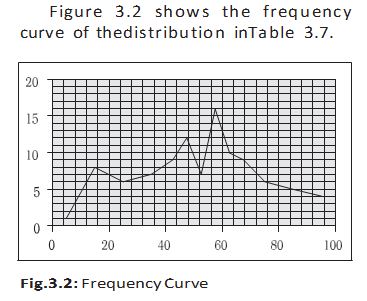
Frequency Array
Frequency array — A classification of data for a discrete variable, showing the frequency corresponding to each value it takes.
Key points
- Discrete values: A discrete variable takes separate values rather than intermediate fractional values between integers.
- Frequency: Count the observations at each value and list the corresponding frequencies.
| Household size | Number of households |
|---|---|
| 1 | 5 |
| 2 | 15 |
| 3 | 25 |
| 4 | 35 |
| 5 | 10 |
| 6 | 5 |
| 7 | 3 |
| 8 | 2 |
| Total | 100 |
Why can unequal class intervals be more suitable than equal intervals?
Quick recap
- Use unequal class intervals when they represent the distribution more appropriately.
- The 40–70 range contains 63 of the 100 students in the example.
- The three central classes are split into classes of width 5; the other classes retain width 10.
- A class mark is the midpoint of its class interval.
- A frequency array lists the frequency at each discrete value.
- Household size is discrete; the example frequency array totals 100 households.
Bivariate Frequency Distribution
Meaning and Purpose
Bivariate frequency distribution — A frequency distribution that shows the frequencies of values or classes for two variables together.
How It Is Organised
- Bivariate data arise when two types of information are collected from each element in a sample.
- Rows and columns represent the classes of the two variables; each cell gives the frequency for the matching pair of classes.
- Use: It summarises the joint distribution of two variables; such distributions are used in studying correlation.
| Advertisement expenditure (thousand Rs) / Sales (lakh Rs) | 115–125 | 125–135 | 135–145 | 145–155 | 155–165 | 165–175 | Total |
|---|---|---|---|---|---|---|---|
| 62–64 | 2 | 1 | — | — | — | — | 3 |
| 64–66 | 1 | — | 3 | — | — | — | 4 |
| 66–68 | 1 | 1 | 2 | 1 | — | — | 5 |
| 68–70 | — | 2 | — | 2 | — | — | 4 |
| 70–72 | — | 1 | 1 | — | 1 | 1 | 4 |
| Total | 4 | 5 | 6 | 3 | 1 | 1 | 20 |
Reading a Cell
- Example: The cell at advertisement expenditure 64–66 thousand Rs and sales 135–145 lakh Rs has frequency 3.
- Meaning: Three of the 20 firms fall in both of those class intervals.
Classification of Data
- Raw data collected from primary or secondary sources are unclassified; classification organises the data for further statistical analysis.
- Frequency distribution groups values into classes and records the corresponding class frequencies.
- Further calculations in a frequency distribution use class marks rather than the original observations.
- Good class formation places each class mark as close as possible to the value around which that class’s observations tend to concentrate.
| Point | Exclusive method | Inclusive method |
|---|---|---|
| Class limits | One limit—upper or lower—is excluded. | Both upper and lower limits are included. |
- Bivariate data
- Data containing two variables recorded for each sample element.
- Cell frequency
- Number of observations belonging to the row and column classes of a cell.
Quick recap
- A bivariate frequency distribution summarises two variables together.
- Rows and columns classify the two variables; each cell records the frequency for a pair of classes.
- In the example, three firms have sales of 135–145 lakh Rs and advertisement expenditure of 64–66 thousand Rs.
- Classification organises raw data for statistical analysis.
- Exclusive classes exclude one limit; inclusive classes include both limits.
- Frequency-distribution calculations use class marks, which should represent where observations in each class tend to concentrate.
Economics — ALL CHAPTERS
1
Introduction
2
Theory of Consumer Behaviour
3
Production And Costs
4
The Theory Of The Firm Under Perfect Competition
5
Market Equilibrium
1
Introduction
2
Collection of Data
3
Organizing of Data
4
Presentation of Data
5
Measures of Central Tendency
6
Correlation
7
Index Numbers
8
Use of Statistical Tools