Class 11 Humanities . Economics . Introductory Micro Economics . The Theory of the Firm Under Perfect Competition
Chapter 4: The Theory Of The Firm Under Perfect Competition
Ch 4
Economics
Class 11 Humanities
Perfect Competition : Defining Features
The Firm’s Objective and Chapter Focus
- Firm’s objective: A firm chooses the level of output that maximises its profit.
- Chapter focus: The chapter analyses profit maximisation, derives a firm’s supply curve and aggregates firms’ supplies to obtain market supply.
Perfect Competition
| Feature | Meaning / implication |
|---|---|
| Many buyers and sellers | Each is small relative to the whole market and cannot influence it through individual size. |
| Homogeneous product | Every firm sells an identical good, so buyers see no difference between firms’ products. |
| Free entry and exit | Firms can enter or leave easily; this supports the existence of many firms. |
| Perfect information | Buyers and sellers know prices, product quality, and other relevant market details. |
Price-Taking Behaviour
Why Firms Take the Market Price
- Many firms sell identical products, and buyers know the market price.
- A firm raises its price above the market price.
- Buyers switch to other firms selling the same good.
- The other firms can readily accommodate them because there are many sellers.
- The firm that raised its price loses all its buyers.
- Homogeneous product
- A good identical across firms, with no product-based distinction for buyers.
- Free entry and exit
- Firms can enter the market or leave it without restriction.
- Perfect information
- Buyers and sellers know relevant prices, quality, and market details.
- Price-taking behaviour
- Accepting the market price rather than setting a price that influences the market.
State the four defining features of perfect competition.
What does price-taking mean for a firm in a perfectly competitive market?
Quick recap
- A firm is assumed to maximise profit and sell all the output it produces.
- A firm’s supply curve shows its chosen output at different market prices.
- The market supply curve is formed by aggregating individual firms’ supply curves.
- Perfect competition has many buyers and sellers, homogeneous products, free entry and exit, and perfect information.
- These features lead buyers and sellers to take the market price as given.
- A firm that charges above the market price loses all its buyers.
Revenue
Revenue and the Price-Taking Firm
Price-taking behaviour
- Price taker: A perfectly competitive firm accepts the market price; it can sell as much as it wishes at that price.
- Selling price: The firm has no reason to charge less than the market price, so it sells at the market price, denoted by .
Total revenue (TR) — The firm’s total earnings from sales, equal to the market price per unit multiplied by the quantity sold.
Here, is the market price and is the quantity produced and sold.
| Boxes sold | Total revenue (Rs.) |
|---|---|
| 0 | 0 |
| 1 | 10 |
| 2 | 20 |
| 3 | 30 |
| 4 | 40 |
| 5 | 50 |
Total revenue curve
- Axes: Output or quantity sold is on the horizontal axis; total revenue is on the vertical axis.
- Shape: Since is constant, is an upward-sloping straight line through the origin.
- Slope: The slope of the TR curve equals the market price, .
Average revenue (AR) — Total revenue earned per unit of output.
For a perfectly competitive firm, average revenue equals the market price.
Price line and the firm’s demand
- Price line: The AR curve is horizontal at , because the price remains constant for every output level.
- Demand curve: The horizontal price line is also the demand curve facing the firm.
- Perfectly elastic demand: The firm can sell any quantity at ; charging more would mean it cannot sell its output.
Marginal revenue (MR) — The increase in total revenue resulting from a one-unit increase in output.
For any output change, the price-taking firm’s marginal revenue is the market price.
Why MR equals price
- Example: Raising candle sales from 2 boxes to 3 increases TR from Rs. 20 to Rs. 30, so MR is Rs. 10—the market price.
- Reason: Each additional unit is sold at the same market price, so the extra revenue from that unit equals .
- Result: Under perfect competition, .
Profit Maximisation
Profit (π) — The firm’s total revenue remaining after its total production cost is subtracted.
is total revenue and is total cost.
Conditions for profit maximisation
- Condition 1: At the profit-maximising output , price equals marginal cost: .
- Condition 2: Marginal cost must be non-decreasing at .
- Condition 3—short run: To continue producing, price must exceed average variable cost: .
- Condition 3—long run: To continue producing, price must exceed average cost: .
Condition 1: Price Equals Marginal Cost
How the profit-maximising condition arises
- If marginal revenue exceeds marginal cost, the extra output adds more to revenue than to cost, so profit rises.
- If marginal revenue is below marginal cost, the extra output adds more to cost than to revenue, so profit falls.
- Maximum profit occurs where .
- For a perfectly competitive firm, , so the condition becomes .
Condition 2: Marginal Cost Must Not Be Falling
Why the MC curve must be non-decreasing
- Intersection alone is insufficient: Price may equal MC at more than one output, but a downward-sloping MC intersection cannot be profit-maximising.
- At : MC is falling. Just below , MC is above price, so reducing output raises profit; therefore, is not a maximum.
- At : An upward-sloping intersection can satisfy the maximisation condition: MC is below price before it and above price after it.
- Total revenue (TR)
- Market price multiplied by quantity sold.
- Average revenue (AR)
- Total revenue per unit; for a price-taking firm, it equals market price.
- Marginal revenue (MR)
- The change in total revenue from an increase in output; it equals price under perfect competition.
- Marginal cost (MC)
- The change in total cost associated with producing an additional unit.
- Price line
- The firm’s horizontal AR and demand curve at the fixed market price.
Why does a perfectly competitive firm have ?
State the conditions for a perfectly competitive firm’s profit-maximising output.
Quick recap
- A price-taking firm sells at the market price and has .
- The TR curve is an upward straight line through the origin with slope .
- For a perfectly competitive firm, ; its demand curve is horizontal.
- Profit equals total revenue minus total cost: .
- Profit maximisation requires , which becomes under perfect competition.
- At the chosen output, MC must be non-decreasing; continued production also requires in the short run or in the long run.
Profit Maximisation
Price Conditions for Positive Output
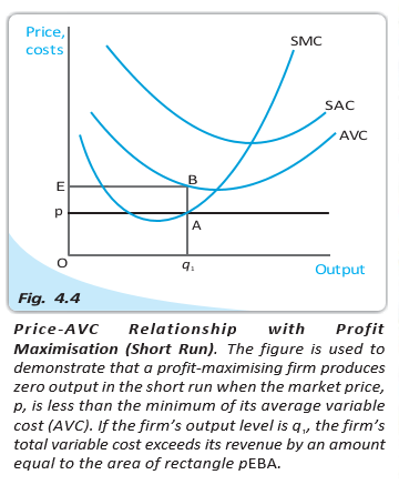
When price is below AVC, the revenue rectangle is smaller than the variable-cost rectangle; the resulting profit is less than the loss from producing zero.
Long-Run Price Condition
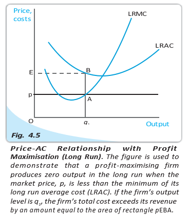
If , total revenue is below total cost, so the firm prefers exit and zero profit.
Graphical Profit Maximisation in the Short Run
The positive-output choice is where the rising short-run marginal cost curve meets market price, subject to the shutdown condition.
At the output shown, total revenue is the price-by-quantity rectangle and total cost is the average-cost-by-quantity rectangle.
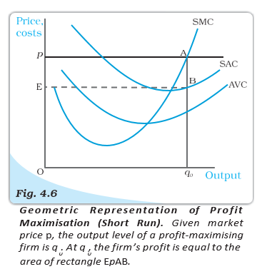
Do not confuse the short-run shutdown test, , with the long-run stay-in-market test, .
Quick recap
- In the short run, producing requires ; below this, the firm shuts down.
- At zero short-run output, revenue and variable cost are zero, so profit is .
- In the long run, the firm stays only when ; otherwise it exits and earns zero profit.
- The competitive firm chooses output where rising equals market price.
- At the chosen output, profit is and appears as the gap between price and average cost.
Supply Curve Of A Firm
Meaning of a Firm’s Supply
- Firm’s supply: The quantity a firm chooses to sell at a given price, with technology and input prices unchanged.
- Representation: A supply schedule lists quantities at different prices; a supply curve shows these choices graphically.
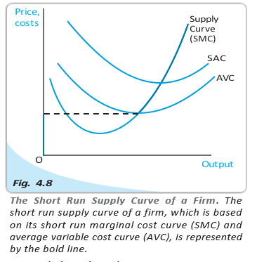
Short-Run Supply Curve
How the Firm Chooses Output
- Profit-maximising output When the firm produces, it chooses output where market price equals the rising part of short-run marginal cost ().
- Production condition The price must also be at least the average variable cost () at that output.
- Shutdown threshold If price is below minimum , every positive output costs more in variable cost than it earns in revenue, so the firm produces zero.
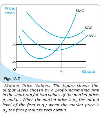
| Market price | Firm’s decision | Reason |
|---|---|---|
| At or above minimum | Produce where price equals rising ; supply that output. | at the chosen output does not exceed price. |
| Below minimum | Produce zero output. | exceeds price at every positive output. |
Short-run supply curve — The rising part of the curve from and above minimum , together with zero output at every price below minimum .
Long-Run Supply Curve
How the Firm Chooses Output
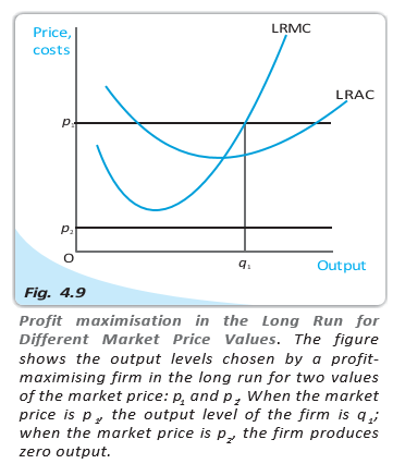
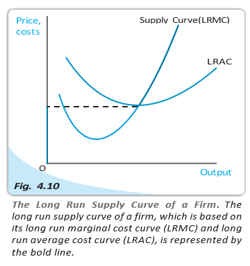
- Profit-maximising output When the firm produces in the long run, it chooses output where market price equals the rising part of long-run marginal cost ().
- Production condition Price must also be at least long-run average cost () at that output.
- Exit threshold If price is below minimum , every positive output has average cost above price, so the firm produces zero.
| Market price | Firm’s decision | Reason |
|---|---|---|
| At or above minimum | Produce where price equals rising ; supply that output. | at the chosen output does not exceed price. |
| Below minimum | Produce zero output. | exceeds price at every positive output. |
Long-run supply curve — The rising part of the curve from and above minimum , together with zero output at every price below minimum .
| Point | Short run | Long run |
|---|---|---|
| Marginal cost curve | Rising | Rising |
| Cost threshold | Minimum | Minimum |
| Zero-output rule | Zero output below minimum | Zero output below minimum |
- Supply schedule
- A table of quantities a firm chooses to sell at different prices, with technology and factor prices fixed.
- Supply curve
- A graph of the firm’s chosen output at different market prices, with other conditions fixed.
- Shutdown threshold
- The minimum average cost level below which the firm chooses zero output in the relevant time period.
What is a firm’s short-run supply curve?
How does the firm’s long-run supply curve differ from its short-run supply curve?
Quick recap
- A firm’s supply is its chosen quantity at a given price, with technology and factor prices fixed.
- When producing, the firm chooses output where price equals the rising marginal cost curve.
- In the short run, positive output requires price to be at least minimum .
- The short-run supply curve is rising from minimum upward, with zero output below it.
- In the long run, positive output requires price to be at least minimum .
- The long-run supply curve is rising from minimum upward, with zero output below it.
The Shut Down Point
The Shut Down Point
Short-run shut down point — The lowest price at which a firm produces positive output in the short run; it occurs at the minimum of AVC, where SMC cuts AVC.
| Period | Shut down point | Production decision |
|---|---|---|
| Short run | Minimum AVC | Produce if price is at least minimum AVC; shut down below it. |
| Long run | Minimum LRAC | Do not produce if price is below minimum LRAC. |
Supply Curve Connection
- Short-run supply: The firm's supply curve is the rising part of SMC at and above minimum AVC; below that price, output is zero.
- Last positive-output point: Moving down the supply curve, production ends at the minimum-AVC point.
Normal Profit and the Break-even Point
Normal profit — The minimum profit needed to keep a firm in its existing business; it is treated as part of the firm's total cost.
Profit and Continuation
- Normal profit: It is the opportunity cost of entrepreneurship; without at least this return, a firm will not remain in business in the long run.
- Super-normal profit: Profit earned over and above normal profit.
- Short run: A firm may continue producing even when its profit is below normal profit, provided it covers the relevant short-run costs.
Break-even point — The point on a firm's supply curve where it earns exactly normal profit.
Break-even Cost Point
- Long run: Break-even occurs where the firm's supply curve intersects LRAC at minimum average cost.
- Short run: The corresponding intersection is with SAC at its minimum.
Opportunity Cost
Opportunity cost — The gain given up from the next-best alternative when a choice is made.
Example: Investing Rs. 1,000
- Alternatives: Keep the money at home for no return, or deposit it in Bank 1 at 10% or Bank 2 at 5%.
- Best forgone option: Bank 1 offers the highest return among the alternatives.
- Opportunity cost: Investing in the family business means giving up the interest available from Bank 1.
Determinants of a Firm's Supply Curve
Link Between Costs and Supply
- Key link: A firm's supply curve is a segment of its marginal cost curve, so factors that change MC also change supply.
- Main factors: Technological progress and input prices affect the firm's costs and therefore its supply.
| Change | Effect on costs / MC | Supply effect |
|---|---|---|
| Technological progress | More output from the same inputs, or the same output from fewer inputs; MC falls. | MC and supply shift right/down; at a given price, output rises. |
| Input price rises | Production costs and usually MC rise. | MC and supply shift left/up; at a given price, output falls. |
Impact of a Unit Tax on Supply
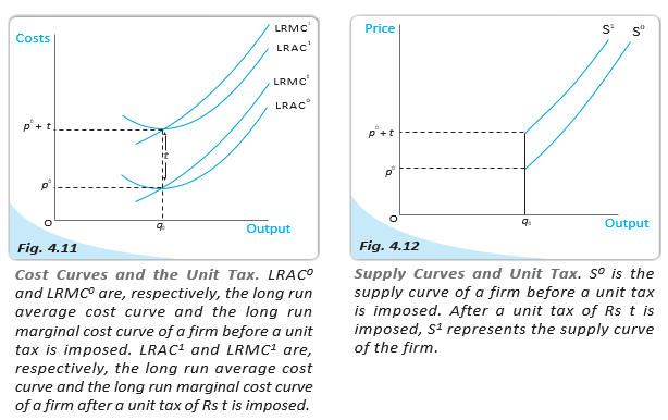
Unit tax — A tax imposed by the government on each unit of output sold.
Tax Effects
- Example: A tax of Rs. 2 per unit on 10 units gives a total tax payment of Rs. 20.
- Costs: A tax of Rs. per unit raises LRAC and LRMC by Rs. at every output level.
- Long-run supply: Since supply is the rising part of LRMC at and above minimum LRAC, the tax shifts the firm's long-run supply curve left.
- Result: At any given market price, the firm supplies fewer units.
The Market Supply Curve
Market supply curve — The total output supplied by all firms in a market at each market price.
Add the output supplied by each firm at the same price.
Horizontal Summation
- Method: At each price, add firms' quantities supplied; graphically, this is the horizontal sum of individual supply curves.
- Two-firm example: If at price firm 1 supplies and firm 2 supplies , market supply is .
- Entry and exit: The market supply curve is derived for a fixed number of firms. More firms shift it right; fewer firms shift it left.
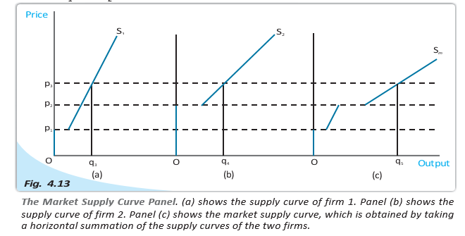
Numerical Market Supply Example
Firm 1 begins supplying at price 10; firm 2 begins at price 15.
Sum the two firms' supply at each price range.
Reading the Example
- Below 10: Neither firm supplies, so market supply is zero.
- From 10 to below 15: Only firm 1 supplies, so market supply equals .
- At 15 and above: Both firms supply, so their quantities add to .
What is the short-run shut down point of a firm?
How is the market supply curve derived from individual firms' supply curves?
Quick recap
- In the short run, a firm shuts down below minimum AVC; in the long run, the shut down threshold is minimum LRAC.
- Normal profit is part of total cost and is the minimum return needed to keep the firm in business.
- Break-even is where the firm earns normal profit at the minimum average-cost point.
- Opportunity cost is the gain sacrificed from the next-best alternative.
- Technological progress shifts supply right; higher input prices and unit taxes shift supply left.
- Market supply is the horizontal sum of firms' supplies at each price; changes in the number of firms shift market supply.
Price Elasticity Of Supply
Meaning and Formula
Price elasticity of supply — It measures how responsive the quantity supplied is to a change in the market price.
It is the percentage change in quantity supplied divided by the percentage change in price. and are the changes in quantity supplied and price; and are their initial values.
Calculating Elasticity
- Example: Cricket-ball output rises from to when price increases from Rs. 10 to Rs. 30.
- Quantity change: Using the old quantity as the base, .
- Price change: Using the old price as the base, .
- Elasticity: .
Elasticity and the Supply Curve
| Supply curve | Elasticity | Reason |
|---|---|---|
| Vertical | Quantity supplied is completely insensitive to price. | |
| Positively sloped | A rise in price is accompanied by a rise in quantity supplied. |
Key Property
- Units: Price elasticity of supply is independent of the units used to measure price and quantity.
Geometric Method for a Straight-Line Supply Curve
Using the Intercepts
- At point : For a straight-line supply curve, elasticity is , where is the quantity-axis intercept, the origin, and the quantity at .
- Negative quantity intercept: If the line cuts the price axis at a positive value and its extension meets the quantity axis at a negative value, ; therefore, at every point.
- Curve through the origin: Here, coincides with , so and at every point.
- Positive quantity intercept: If the line meets the quantity axis at a positive value, ; therefore, at every point.
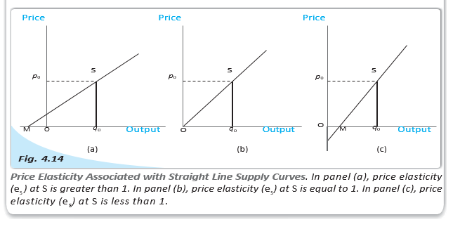
Price rises from Rs. 10 to Rs. 30, while quantity supplied rises from 200 to 1,000. Find price elasticity of supply.
What is the elasticity of a straight-line supply curve that passes through the origin?
Quick recap
- Price elasticity of supply is the percentage change in quantity supplied divided by the percentage change in price.
- For the cricket-ball example, elasticity is .
- A vertical supply curve has zero elasticity; a positively sloped supply curve has positive elasticity.
- Elasticity is independent of measurement units.
- For a straight-line supply curve, a negative quantity intercept implies elasticity greater than , an origin intercept implies elasticity equal to , and a positive quantity intercept implies elasticity less than .
Economics — ALL CHAPTERS
1
Introduction
2
Theory of Consumer Behaviour
3
Production And Costs
4
The Theory Of The Firm Under Perfect Competition
5
Market Equilibrium
1
Introduction
2
Collection of Data
3
Organizing of Data
4
Presentation of Data
5
Measures of Central Tendency
6
Correlation
7
Index Numbers
8
Use of Statistical Tools