Class 11 Humanities . Economics . Statistics For Economics . Presentation of Data
Chapter 4: Presentation of Data
Ch 4
Economics
Class 11 Humanities
Introduction
Why Present Data?
Presentation of data — Organising collected data into a form that is compact, clear and easy to understand and use.
Main forms
- Textual or descriptive: Data are explained in sentences.
- Tabular: Data are arranged in rows and columns.
- Diagrammatic: Data are represented using diagrams.
Textual Presentation of Data
Textual presentation — A form of presentation in which data are described within written text.
When it is useful
- Suitable when: The amount of data is not large.
- Advantage: Written description can emphasise selected points.
- Drawback: Readers must go through the full text to understand and compare the data.
Examples
- Bihar bandh, 8 September 2005: Of 22 petrol pumps, 5 were open and 17 closed; of 11 schools, 2 were closed and 9 open.
- Census of India 2001: Population was 102 crore—53 crore males and 49 crore females; 74 crore lived in rural areas and 28 crore in towns or cities.
- Workers: There were 40 crore workers and 62 crore non-workers nationally. Urban areas had 9 crore workers and 19 crore non-workers; rural areas had 31 crore workers.
Tabular Presentation of Data
Tabular presentation — A form of presentation in which data are arranged in rows (horizontal) and columns (vertical).
Structure and use
- Cell: A box at the intersection of a row and a column; it gives information by relating the row and column categories.
- Example: A table has 3 rows, 3 columns and 9 cells.
- Advantage: Tabulation organises data for further statistical treatment and decision-making.
| Sex | Rural | Urban | Total |
|---|---|---|---|
| Male | 79 | 90 | 82 |
| Female | 59 | 80 | 65 |
| Total | 68 | 84 | 74 |
Four kinds of classification
- Qualitative: By attributes or qualities.
- Quantitative: By measurable numerical characteristics.
- Temporal: By time.
- Spatial: By place or location.
Qualitative Classification
Qualitative classification — Classification of data according to attributes or qualities rather than numerical measurements.
Examples
- Possible attributes: Social status, physical status and nationality.
- Literacy table: Sex (male, female, total) and location (rural, urban, total) are the qualitative classification attributes.
- Data source: Census of India 2011; literacy rates are for people aged 7 years and above.
Quantitative Classification
Quantitative classification — Classification based on characteristics that can be measured numerically.
Key points
- Examples of measurable characteristics: Age, height, production and income.
- Class limits: The lower and upper values that define the boundaries of a class or group.
- Example: Respondents are grouped into age intervals such as 20–30 years and 30–40 years.
Use this to find the percentage for an age group.
| Age group (years) | Respondents | Per cent |
|---|---|---|
| 20–30 | 3 | 0.55 |
| 30–40 | 61 | 11.25 |
| 40–50 | 132 | 24.35 |
| 50–60 | 153 | 28.24 |
| 60–70 | 140 | 25.83 |
| 70–80 | 51 | 9.41 |
| 80–90 | 2 | 0.37 |
| All | 542 | 100.00 |
Example calculation
- Missing frequency: respondents.
- Missing percentage: .
Temporal Classification
Temporal classification — Classification in which time is the classifying variable.
Key points
- Time units: Hours, days, weeks, months or years.
- Example: A tea shop's annual sales are classified by year.
| Year | Sales (Rs. in lakhs) |
|---|---|
| 1995 | 79.2 |
| 1996 | 81.3 |
| 1997 | 82.4 |
| 1998 | 80.5 |
| 1999 | 100.2 |
| 2000 | 91.2 |
Spatial Classification
Spatial classification — Classification of data according to place or location.
Key points
- Possible places: Village, town, block, district, state or country.
- Example: India's exports can be classified by destination.
| Destination | Export share |
|---|---|
| USA | 12.5 |
| Germany | 2.4 |
| Other EU | 10.9 |
| UK | 3.1 |
| Japan | 2.2 |
| Russia | 0.7 |
| China | 4.7 |
| West Asia – Gulf Cooperation Council | 15.3 |
| Other Asia | 29.4 |
| Others | 18.8 |
| All | 100.0 |
What are the four kinds of classification used in tabulation?
State one advantage and one drawback of textual presentation.
Quick recap
- Data are presented textually, in tables or diagrammatically to make them easier to use and understand.
- Textual presentation suits small amounts of data; it is descriptive but can be difficult to compare quickly.
- Tables organise information in rows and columns; each intersecting box is a cell.
- Tabulation uses qualitative, quantitative, temporal or spatial classification.
- Qualitative data describe attributes; quantitative data use measurable characteristics grouped by class limits.
- Temporal classification groups by time, while spatial classification groups by place.
Tabulation Of Data And Parts Of Data
Tabulation and Classification
Tabulation — The systematic presentation of data in rows and columns, with explanatory details, to make it easier to understand.
Classification by number of characteristics
- One-way classification: Data are classified by one characteristic.
- Two-way classification: Data are classified by two characteristics.
- Three-way classification: Data are classified by three characteristics.
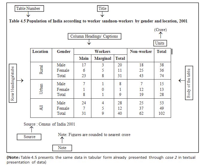
Parts of a Statistical Table
| Part | Function and placement |
|---|---|
| Table number | Identifies and distinguishes a table; placed at the top or before the title. Numbers are usually whole numbers in ascending order. A number such as 4.5 can identify the fifth table in Chapter 4. |
| Title | Briefly and clearly states the table’s contents; placed after or below the table number. |
| Captions / column headings | Name the columns and explain the figures shown in them. |
| Stubs / row headings | Name the rows. The complete left-hand column of row headings is the stub column. |
| Body | The main part containing the data. Each value is located by its row and column. |
| Unit of measurement | State the unit with the title; if units differ across rows or columns, state them with the relevant stubs or captions. Round off large figures and indicate the rounding method. |
| Source | Briefly identifies where the data came from; usually written below the table. If there are multiple sources, list all of them. |
| Note | Explains a specific feature of the data that is not self-explanatory and has not been explained elsewhere; placed last. |
Reading a table cell
- Locate data: Read a value using both its row heading and column heading.
- Example: In the cited table, the second row and fourth column give 25 crore females in rural India who were non-workers in 2001.
- Caption
- A column heading that describes the figures in that column.
- Stub
- A row heading; the full left-hand row-heading column is the stub column.
- Body
- The section of a table containing the actual data.
- Source
- A brief statement identifying the origin of the table’s data; list all sources when there is more than one.
- Note
- A final explanation of a data feature that is not clear from the table itself.
Differentiate between captions and stubs.
Quick recap
- Tabulation presents data systematically in rows and columns.
- Classification may be one-way, two-way or three-way, according to the number of characteristics.
- A table’s number and title identify it and describe its contents.
- Captions label columns; stubs label rows; the body contains the data.
- State measurement units clearly; round off large figures and indicate the rounding method.
- List every data source below the table; place any explanatory note last.
Diagramatic Presentation Of Data
Purpose and Types of Diagrams
Diagrammatic presentation — A visual method of presenting data that makes numerical information quick to understand.
- Strength: Diagrams turn abstract numbers into a concrete, easily understood form and often communicate faster than tables or text.
- Limitation: Diagrams may be less accurate than tables, but are often more effective for quick understanding.
- Main types: Geometric diagrams, frequency diagrams and arithmetic line graphs.
- Geometric diagrams: Include bar diagrams and pie diagrams; bar diagrams may be simple, multiple or component.
Bar Diagrams
Bar diagram — A diagram made of equally spaced, equal-width rectangular bars whose height or length represents the value of each category.
- Baseline: Each bar starts at zero; compare categories by their relative bar heights or lengths.
- Data: Suitable for frequency and non-frequency data, including discrete variables and attributes.
- Examples: Family size, dice scores, examination grades, gender, religion, population, production and income–expenditure data.
- Time series: Bars commonly compare values across years, such as food-grain production or literacy rates.
- Interpretation: A longer bar means a greater measured or counted value.
| Type | What it shows | Example |
|---|---|---|
| Simple bar | One value for each category | Literacy rates across states |
| Multiple bar | Two or more related data sets side by side | Imports and exports across years |
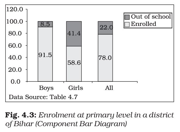
| Component bar | A total divided into its component parts | Enrolled and out-of-school children |
Multiple Bar Diagrams
- Purpose: Compare two or more sets of data for the same categories.
- Examples: Income versus expenditure, imports versus exports, or marks in different subjects.
Component Bar Diagrams
- Purpose: Show both the total and the relative sizes of its component parts.
- Construction: Draw a bar for the total, then divide it into components in proportion to their values.
- Percentage data: Make each total bar 100 units high, then mark component heights equal to their percentages.
- Other data: Scale the bar to the total value and calculate each component’s proportional height.
- Presentation: Shade or colour components distinctly; give smaller components priority when dividing the bar.
| Group | Enrolled | Out of school |
|---|---|---|
| Boys | 91.5% | 8.5% |
| Girls | 58.6% | 41.4% |
| All children | 78.0% | 22.0% |
Reading Bar-Diagram Comparisons
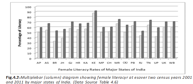
- Example finding: Female literacy increased across the country between the two census years shown.
- State comparison: Bihar, Jharkhand and Uttar Pradesh had some of the sharpest rises in female literacy.
Pie Diagrams
Pie diagram — A circular component diagram in which the circle is divided into sectors proportional to the parts of a whole.
- Whole circle: Represents 100% or , regardless of the circle’s radius.
- Categories: Each component is shown as a sector; its central angle is proportional to its share of the total.
- Preparation: Convert each component’s absolute value into a percentage of the total before finding its sector angle.
- Link to component bars: The same component data can be shown in either form, but pie-chart values must be converted to percentages first.
Use these formulas for component value , total , percentage , and sector angle .
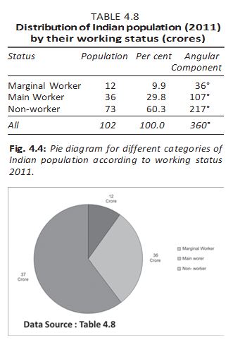
Do not use absolute component values directly as pie-chart angles: first divide each value by the total, convert to a percentage, and then multiply by .
Quick recap
- Diagrams communicate data quickly, though they may be less precise than tables.
- Bar diagrams use equal-width, equally spaced bars that begin at zero; bar height or length shows magnitude.
- Bar diagrams can show frequency and non-frequency data, including discrete variables and attributes.
- Simple bars show one series, multiple bars compare series, and component bars divide totals into parts.
- For percentage data, component bars have a total height of 100 units; otherwise scale the bar to the total and calculate proportional component heights.
- For a pie chart, convert each absolute value to a percentage of the total, then use .
Frequency Diagram
Frequency diagrams — Graphs used to present grouped frequency distributions include histograms, frequency polygons, frequency curves and ogives.
Histogram
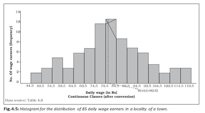
Histogram — A two-dimensional diagram of adjacent rectangles for a continuous frequency distribution, with class intervals on the X-axis and frequencies represented by rectangle areas.
How to read a histogram
- Class intervals: The horizontal base of each rectangle spans the class boundaries; its height is set so its area represents the class frequency.
- Equal widths: When class intervals have equal widths, rectangle heights are proportional to frequencies, making direct comparison straightforward.
- Unequal widths: Compare areas, not raw heights. Use frequency density as the rectangle height.
- Frequency density: Calculate it by dividing class frequency by class-interval width: .
- Continuity: Rectangles touch because class boundaries are continuous. Convert discontinuous classes into continuous classes before drawing.
- Mode: The histogram can show the mode graphically; the horizontal coordinate of the indicated vertical line gives the modal value.
| Point | Histogram | Bar diagram |
|---|---|---|
| Data type | Used for continuous variables | Can be used for discrete or continuous variables |
| Spacing | Rectangles are adjacent; no gaps between consecutive classes | Gaps are left between consecutive bars, except in multiple or component bar diagrams |
| What represents the data | Width and height both matter; area represents frequency | Height matters; bar width and area are arbitrary |
Frequency Polygon
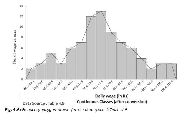
Frequency polygon — A grouped frequency distribution shown by joining plotted class-frequency points with straight-line segments; it can be drawn from or instead of a histogram.
Constructing and using one
- Plotting: Plot each class frequency against its class midpoint; class boundaries or class marks may be shown on the X-axis.
- Class mark: The midpoint of a class interval is .
- Joining points: Join consecutive plotted points with short straight lines.
- Closing the polygon: Add a zero-frequency class midpoint just before and after the distribution, then join both ends to the baseline. This makes the area under the polygon represent total frequency or sample size.
- Comparing distributions: Polygons are often clearer than overlaid histograms because bars from different distributions can coincide.
Frequency Curve
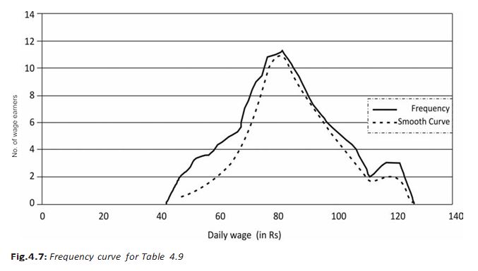
Frequency curve — A smooth, freehand curve drawn through or close to the points of a frequency polygon.
- Shape: The smooth curve need not pass through every polygon point; it should follow the overall pattern as closely as possible.
Ogive
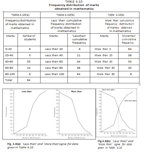
Ogive — A cumulative frequency curve formed by plotting cumulative frequencies against the relevant class limits.
| Type | Plot cumulative frequency against | Direction |
|---|---|---|
| Less-than ogive | Upper class limits | Never decreases |
| More-than ogive | Lower class limits | Never increases |
- Median: The intersection point of the less-than and more-than ogives gives the median of the distribution.
Arithmetic Line Graph
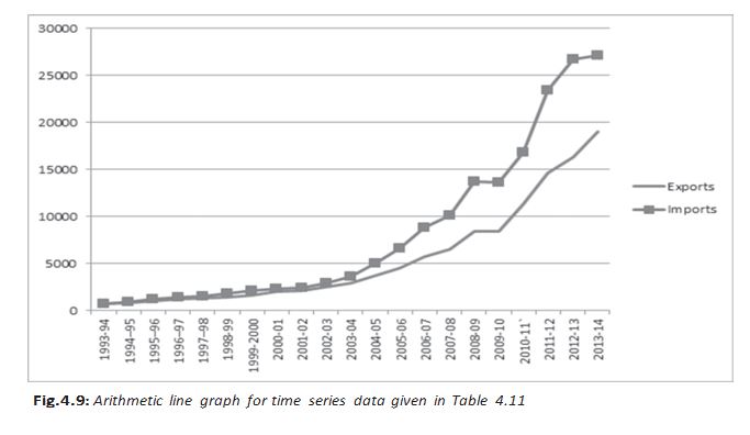
Arithmetic line graph — A time-series graph with time on the X-axis and the variable's values on the Y-axis; plotted points are joined by lines.
Purpose and example
- Time scale: The X-axis may show hours, days, dates, weeks, months or years.
- Use: It helps reveal trends and periodic patterns in long-term time-series data.
- India's trade: From 1993–94 to 2013–14, imports remained above exports. Both rose rapidly after 2001–02, and the gap widened.
Why is frequency density used for a histogram with unequal class widths?
How does a frequency polygon differ from a frequency curve?
What does the intersection of two ogives show?
Quick recap
- A histogram represents class frequencies by rectangle areas; use frequency density when class widths differ.
- Histogram rectangles touch and are used for continuous variables; bar diagrams have gaps and rely on bar height.
- A frequency polygon joins frequency points and can help compare distributions; a frequency curve smooths its shape.
- Less-than ogives use upper class limits and do not decrease; more-than ogives use lower class limits and do not increase.
- The intersection of less-than and more-than ogives gives the median.
- Arithmetic line graphs plot time against values to show trends and periodic patterns.
Economics — ALL CHAPTERS
1
Introduction
2
Theory of Consumer Behaviour
3
Production And Costs
4
The Theory Of The Firm Under Perfect Competition
5
Market Equilibrium
1
Introduction
2
Collection of Data
3
Organizing of Data
4
Presentation of Data
5
Measures of Central Tendency
6
Correlation
7
Index Numbers
8
Use of Statistical Tools