Class 8 . Mathematics . Ganita Prakash Part II . Tales By Dots and Lines
Chapter 5: Tales by Dots and Lines
Ch 5
Mathematics
Class 8
The Balancing Act
Mean as the Balance Point
At the mean, the total distance from values below it equals the total distance from values above it. This balance occurs at only one value.
Use the first formula for any data set; the second shows why the mean of two values is their midpoint.
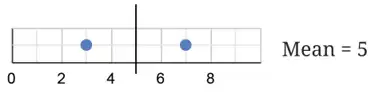
Check the balance around a mean
- Find the mean of the values.
- Add the distances from values below the mean.
- Add the distances from values above the mean; the two totals match.
Show that is the balance point of .
- Find the mean of .
- Total distance below the mean is .
- The value above the mean is , at distance .
Do not assume the mean is the midpoint of the smallest and largest values. Check the total distances on both sides instead.
How Adding or Removing a Value Changes the Mean
Adding a value above the current mean raises the mean; adding one below lowers it. Adding a value equal to the mean leaves it unchanged.
Removing a value below the mean raises the mean; removing one above lowers it. Removing a value equal to the mean leaves it unchanged.
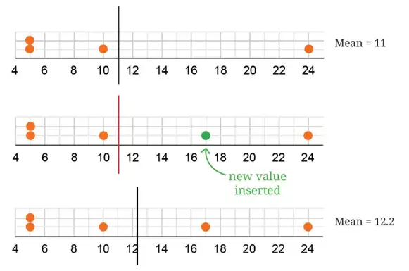
Predict the effect of a data change
- Compare the added or removed value with the current mean.
- For adding, use the total of the old data plus , divided by the new count.
- For removing, subtract from the old total and divide by the remaining count.
Predict and calculate how the mean changes when a value is added or removed.
- The data have mean .
- Adding , which is above the mean, raises it.
- Removing , which is below the mean, also raises it.
- Adding a value equal to the mean keeps the mean unchanged.
The values are . Find their mean and verify the balance property.
A data set of values has mean . What is the new mean after adding ?
- Median: The middle value after arranging data in order; it is distinct from the mean.
- Balance: At the mean, total distances below and above are equal.
- Change: Adding a value above the mean raises it; removing a value below the mean raises it.
Quick recap
- The mean is the total of the values divided by their count.
- For two values, the mean lies halfway between them.
- For any data set, the mean balances total distances on its two sides.
- The balance point is unique and is not always the midpoint of the extremes.
- Adding a value above or below the mean shifts the mean in the same direction.
- Removing a value below or above the mean shifts the mean in the opposite direction.
Balancing act – Unchanging & Relatively Unchanged Mean
Keeping the Mean Unchanged
For an original mean , values added or removed must have a total of , where is the number of those values. Equivalently, their deviations from must sum to zero.
How values balance around the mean
- Below and above: Values below the mean can be balanced by values above it if their total deviations cancel.
- Example: For mean , the added values keep the mean unchanged because their sum is .
- Removal: Removing values with mean equal to the original mean also leaves the remaining mean unchanged.
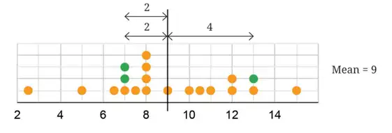
Use this condition for a group of added or removed values.
Check whether the mean stays the same
- Find the original mean, , by dividing the original sum by the number of original values.
- Find the sum of the values being added or removed.
- The mean stays unchanged exactly when the group mean is .
A collection has mean . Does adding and change its mean?
- A collection has mean . Check whether adding and keeps its mean unchanged.
- The added values have mean , so they balance around the original mean.
Adding or Subtracting the Same Number
If the original mean is , adding to every value gives mean ; subtracting gives mean .
Use for addition to every value and for subtraction from every value.
The data are . Find the mean after adding to every value, then subtracting from each result.
- Find the mean of the given values.
- Adding to every value increases the mean by .
- Subtracting from each of those shifted values lowers that mean by .
Multiplying Every Value by the Same Number
If each of values is multiplied by , the new mean is times the old mean.
For example, doubling every value doubles the mean.
The mean of a data set is . Find the new mean if every value is doubled.
- The original data have sum and values, so their mean is .
- Doubling every value doubles the mean.
Do not add or subtract a fixed number only once from the total: if there are values, the total changes by , so the mean changes by .
A data set has mean . Does adding keep the mean unchanged?
A collection has mean . What is its new mean if is subtracted from every value?
The mean of a collection is . Find the new mean if every value is multiplied by .
Quick recap
- The mean stays unchanged when added or removed values have mean equal to the original mean.
- Values on opposite sides of the mean balance when their deviations sum to zero.
- Adding to every value adds to the mean.
- Subtracting from every value subtracts from the mean.
- Multiplying every value by multiplies the mean by .
Balancing Act – Tinkering with median
How Adding a Value Affects the Median
For an odd number of values, take the central value. For an even number, take the mean of the two central values.
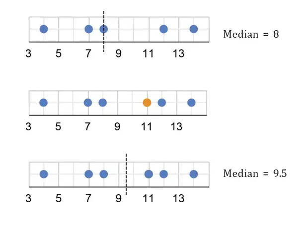
Use this when the ordered data has an even number of values.
Find the New Median
- Arrange the original data in order and identify its median.
- Insert the new value and locate the middle position or positions again.
- If there are an even number of values, average the two middle values.
After adding a value, the two middle values are and . Find the new median.
- After adding , the two middle values in the ordered data are and .
- Average the two middle values.
Finding an Unknown Value from the Mean
Use this relationship to find a missing value when the mean and number of values are known.
Find a Missing Data Value
- Multiply the mean by the number of values to find their total.
- Add the known values.
- Subtract the sum of the known values from the total.
Nine player weights are kg. The mean weight of all ten players is kg. Find the missing weight.
- Find the total weight of the ten players.
- Add the nine recorded weights.
- Subtract the known total from the full total.
Correcting a Mean After an Error
Use when one value was recorded units more than its actual value.
Correct the Mean
- Multiply the original mean by the number of items to find the recorded total.
- Subtract the amount of over-recording to find the actual total.
- Divide the actual total by the number of items.
The recorded average harvest is coconuts per tree for trees. One tree’s count was recorded coconuts too high. Find the corrected average.
- Find the total implied by the original mean for trees.
- Subtract the coconuts that were over-recorded.
- Divide the corrected total by the number of trees.
The mean of numbers is . Seven numbers add up to . Find the eighth number.
The average recorded count for plants is . One count was recorded higher than its actual value. Find the corrected average.
Do not adjust the mean directly for an error in one data value; first correct the total, then divide by the number of values.
Quick recap
- The median is the central value, or the average of the two central values for an even-sized data set.
- Adding a value changes the data’s middle position, so reorder the data and recalculate its median.
- Mean equals the total of values divided by the number of values.
- Find a missing value by subtracting the known-value sum from the total implied by the mean.
- For an over-recorded value, subtract the excess from the recorded total before finding the corrected mean.
Balancing Act – Mean and median with frequencies
Mean from a Frequency Table
Use this when each distinct value has a listed frequency.
Find the Mean from Frequencies
- Multiply each value by its frequency.
- Add the products and add the frequencies.
- Divide the sum of products by the total frequency.
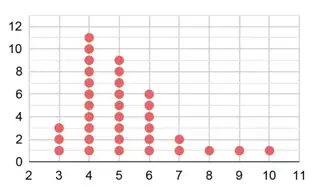
Find the mean family size from the table.
- Multiply each family size by its frequency, then add the products.
- Add the frequencies to find the total number of students.
- Divide the total of the values by the number of students.
Do not average only the distinct values. Include repeats by multiplying each value by its frequency.
Median from a Frequency Table
If a value's cumulative frequency first reaches or exceeds a position, that value occupies that position in the ordered data.
Find the Median from Frequencies
- Add the frequencies to get the total number of observations.
- Find the middle position or positions, depending on whether the total is odd or even.
- Use cumulative frequencies to identify the values at those positions.
- For an even total, average the two middle values.
Find the median family size from the frequency table.
- There are 36 observations, so the middle positions are 18 and 19.
- The cumulative frequency is 14 at family size 4 and 23 at family size 5; thus positions 15 through 23 contain 5.
- Both middle values are 5, so their average is 5.
Do not choose the middle distinct value in the table. Find the middle position(s) among all observations using cumulative frequencies.
Find the mean for values 2, 4, 6 with frequencies 2, 3, 1 respectively.
Find the median for values 1, 2, 3 with frequencies 1, 4, 2 respectively.
Quick recap
- Mean for frequency data: multiply each value by its frequency, add the products, and divide by total frequency.
- The total number of observations is the sum of all frequencies.
- The median is found from the middle position(s) in the ordered data.
- Cumulative frequency reveals which value occupies a given position.
- For an even number of observations, average the values at the two middle positions.
Balancing Act - Spreadsheet
Spreadsheets
Spreadsheet — A spreadsheet is a digital grid of cells arranged in rows and columns, used to enter and calculate with data.
Spreadsheet structure
- Cells can contain text, numbers or formulas.
- Cell reference combines a column letter and row number; Farooq’s Mathematics mark is in cell .
- Reading cells: contains Gowri’s Odia mark, ; Ashwin scored above in Telugu, English and Mathematics.
- Range: write the first and last cells separated by a colon; represents Nagesh’s subject marks, while represents the first five students’ English marks.
| Function | Use | Example |
|---|---|---|
| SUM | Adds the values in a range. | |
| AVERAGE | Finds the mean of the values in a range. |
Entering a spreadsheet formula
- Select the cell where the result should appear.
- Type an equals sign, the function name and the cell range.
- Press Enter to display the result.
Applying spreadsheet formulas
- Science class average: type when the students’ data occupies rows –.
- Subject averages: use for Odia and for Telugu, then compare the results.
- Totals by student: enter a row-sum formula such as in the first student’s Total cell and use the corresponding row range for each student.
- Averages below the data: use the corresponding subject column range, such as for Odia.
Find Nagesh’s total marks using the spreadsheet formula.
- Nagesh’s marks are in the range ; add the six subject marks.
- Enter the spreadsheet formula in the Total cell.
Mean (Average)
Mean — The mean is the total of all data values divided by the number of values.
Use this formula to find the average of a data set.
Adding to every value increases the mean by ; subtracting from every value decreases it by . For evenly spaced values, the mean is the average of the first and last values.
Finding a mean
- Add all the data values.
- Count the values.
- Divide the sum by the count.
Find the means of the first natural numbers, the first odd numbers and the first multiples of .
- The first natural numbers run from to .
- The first odd numbers run from to .
- The first multiples of run from to .
The mean height of students measured in shoes is . The shoes add to every measurement. Find the correct mean height.
The mean of is . Find .
Median
Median — The median is the middle value when the data is arranged in ascending or descending order.
Arrange the data in order first. For an even number of values, average the two middle values.
Finding a median
- Arrange the values in order.
- Locate the middle value, or the two middle values if the count is even.
- For an even count, average the two middle values.
Find the median of .
- The list is already in order and has values, so use the th and th values.
- The middle values are and ; average them.
The numbers of students taking to trials to hit a bull’s eye are . Find the minimum, maximum, mean and median number of trials.
Quick recap
- A spreadsheet stores text, numbers and formulas in cells named by column and row.
- A range such as identifies a sequence of cells.
- totals a range; finds its mean.
- Mean equals the sum of the values divided by the number of values.
- Adding the same amount to every value changes the mean by that amount.
- Find the median by ordering the data and locating its middle value or values.
Visualizing and Interpreting Data
Line Graphs
Line graph — A graph in which data points are connected by lines to show how values change, often over time.
How to read a line graph
- Use: Line graphs are useful for showing how data changes across time.
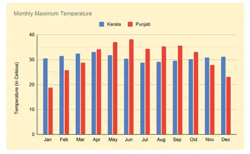
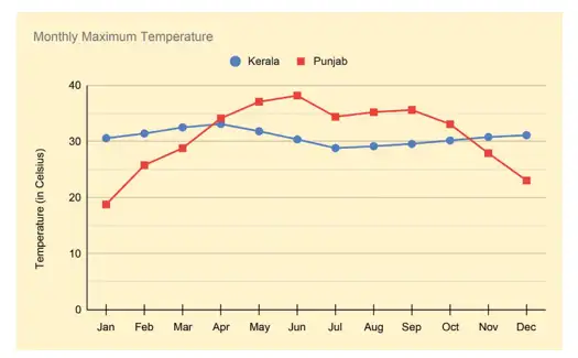
- Axes: The horizontal axis shows the months; the vertical axis shows temperature in degrees Celsius.
- Lines: Each month’s value is marked and connected to the next; colours or symbols distinguish different data sets.
- Monthly maximum: For a state, it is the highest temperature among the values recorded across its weather stations.
Identifying the graph's data
- Kerala: Its monthly data is shown with blue circle marks connected by blue lines.
- Punjab: Its monthly data is shown in red.
- Representation: The clustered-column graph and line graph represent the same information in different forms.
Interpreting Data and Trends
Two steps for interpreting a graph
- Identify: Check what the graph shows, its axes and scale, and how each data set is marked.
- Infer: Describe rises, falls, peaks, low points, and comparisons; then state a conclusion supported by the graph.
Use the range to compare how much the values vary.
Compare the monthly maximum-temperature trends in Punjab and Kerala.
- In Punjab, the monthly maximum rises from January to June, then falls to just under in July, stays mostly level through September, and then falls continuously to December.
- In Kerala, temperatures stay mostly steady, with a peak in April and a low point in July.
- Compare the ranges to see which state varies more.
What the temperature graph shows
- Punjab: The monthly maximum rises from about in January to about in June; it falls to just under in July, stays mostly level through September, then drops continuously to about in December.
- Kerala: Temperatures stay mostly steady; the peak is about in April and the low is about in July.
- Conclusion: Punjab has a wider range, with colder winter and warmer summer monthly maximum temperatures than Kerala.

Which state shows greater variation in monthly maximum temperatures, and what evidence supports your answer?
What does the horizontal axis show in the monthly temperature line graph, and what does the vertical axis show?
Quick recap
- Line graphs connect data points to show changes, often over time.
- In the temperature graph, months are on the horizontal axis and degrees Celsius are on the vertical axis.
- Kerala is marked with blue circles and lines; Punjab is shown in red.
- A state's monthly maximum temperature is the highest value among recordings across its weather stations.
- Identify the graph's variables, scale, and markings before interpreting its trends.
- Punjab's monthly maximum temperatures vary more than Kerala's in the example.
Visualizing and Interpreting Data- Space Jam
Reading and Interpreting Line Graphs
Interpreting the Space-Launch Graph
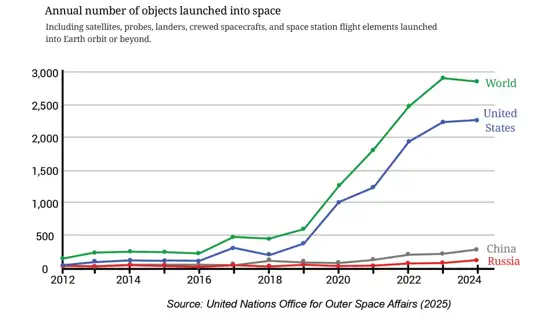
- Worldwide count: It is about 2,900 in 2023 and 2,800 in 2024, so it did not increase every year.
- Highest shown value: 2023 is higher than 2024 and is the highest in the displayed period, assuming the earlier trend was decreasing.
- Other countries: The USA, China, and Russia do not add up to the worldwide total, so other countries are included in the total.
- USA change: Its increase from 2022 to 2023 is greater than from 2023 to 2024; the first rising segment is steeper.
- USA share: In 2022–2024, the USA accounts for about three-quarters of the worldwide count.
- China and Russia: Their combined launch count in 2024 is about 400.
- Nepal: The graph cannot show that Nepal launched no objects; Nepal's data may simply not be displayed.
- At least twofold increase: The worldwide count increased by two times or more from 2019 to 2020.
Read and Interpret a Line Graph
- Read the axis labels, units, and scale.
- Read the values at the points you need to compare.
- Use the direction and steepness of the segment to describe change.
- Check that the graph includes the information needed to support your conclusion.
| Point | Line graph | Clustered column graph |
|---|---|---|
| Best suited for | Showing changes and trends over time | Comparing groups of values |
| Space-launch data | Makes yearly trends easy to follow | Would have 13 clusters and 52 bars, making it crowded and harder to interpret |
Comparing Monthly Rainfall
Average the rainfall measurements for the same month across the years.
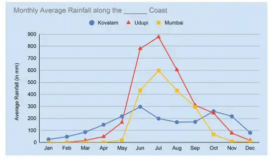
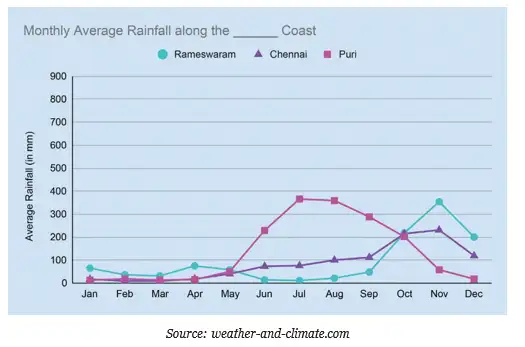
Coastal Grouping and Rainfall Patterns
- West coast: Kovalam, Udupi, and Mumbai are along India's west coast.
- East coast: Rameswaram, Chennai, and Puri are along the east coast.
- Broad pattern: The graphs suggest that west-coast regions receive more rain, though individual cities have different peak months.
- Monsoons: Seasonal rainfall patterns can be considered alongside the south-west and north-east monsoons and the regions they influence.
| City | Peak rainfall | Low rainfall |
|---|---|---|
| Udupi | June–August | January–March |
| Mumbai | June–August | January–March |
| Kovalam | June–August | January–March |
| Rameswaram | October–December | Very little rain from January–September |
| Chennai | Rain begins in June, peaks in November, and continues through December | January–March |
| Puri | July–September | January–March |
Plotting and Reading Data
| Activity | Mon | Tue | Wed | Thu | Fri | Sat | Sun |
|---|---|---|---|---|---|---|---|
| Visiting | 16 | 19 | 10 | 14 | 20 | 22 | 35 |
| Purchasing | 10 | 8 | 7 | 11 | 12 | 16 | 26 |
Plot Two Data Series on One Line Graph
- Put the categories, such as weekdays, on the horizontal axis and the counts on the vertical axis.
- Choose a suitable scale and plot each series as a separate set of points.
- Join each series in order and label the lines clearly.
- Compare the lines to describe similarities and differences.
How should the weekly shop data be shown on a line graph, and what pattern does it show?
- Plot the visiting-customer values in Monday-to-Sunday order.
- Plot the purchasing-customer values as a second series on the same axes.
- Join and label each series; both reach their highest value on Sunday.
- Visitors outnumber purchasers on every day.
| City | Jan | Feb | Mar | Apr | May | Jun | Jul | Aug | Sep | Oct | Nov | Dec |
|---|---|---|---|---|---|---|---|---|---|---|---|---|
| Mangaluru | 0.1 | 0 | 0.1 | 1.8 | 6.2 | 24.1 | 27.7 | 24.5 | 14 | 8.8 | 3.9 | 0.9 |
| Port Blair | 2.4 | 1.3 | 0.9 | 3.3 | 15.5 | 18.7 | 17.3 | 18.8 | 16.8 | 14.1 | 11.3 | 5.4 |
| Rameswaram | 2.6 | 1.3 | 1.9 | 3.4 | 2.5 | 0.4 | 1 | 1 | 1.9 | 8.1 | 10.4 | 7.8 |
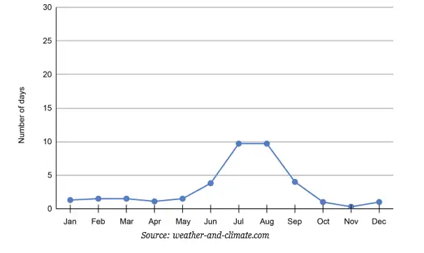
Add the average rainy days for all 12 months to compare annual totals.
Plotting and Interpreting Rainy-Day Data
- Measure: The table records average rainy days per month, not rainfall amounts.
- Plotting: Put months on the horizontal axis and rainy-day counts on the vertical axis; plot each city as a separate line.
- Rounding: For plotting, round values to the nearest integer.
- New Delhi: Read its monthly values from the provided graph and enter them in the table.
- Seasons: Use the monthly patterns to identify each city's rainy season; read the graph scale rather than guessing.
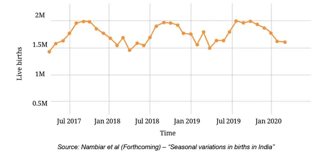
Read a Multi-Year Graph
- For one month in one year, find the month and follow the correct year line to its point.
- To compare the same month across years, compare the corresponding points on those year lines.
- Estimate a yearly total by adding the monthly values for that year.
- State approximate readings as estimates, using the graph's scale.
The worldwide launch count was about 2,900 in 2023 and 2,800 in 2024. Did it increase every year? Name a consecutive-year pair in which it increased by at least two times.
Using the rainy-day table, which of Mangaluru, Port Blair, and Rameswaram has the greatest and least annual total?
A graph shows the USA, China, and Russia, but their combined count is below the worldwide total. What can you infer about other countries, and what can you conclude about Nepal?
For graph-based answers, identify the scale and mark conclusions as approximate when appropriate; never treat missing data as zero.
Quick recap
- Read axes, units, and scale before interpreting a line graph.
- A steeper rising segment means a greater increase between consecutive points.
- The worldwide launch count doubled or more from 2019 to 2020, then fell from 2023 to 2024.
- A graph supports conclusions only about the data it includes; missing data is not zero.
- Monthly average rainfall is found by averaging each month's totals across years.
- Rainfall peaks vary by city, and rainy-day counts are different from rainfall amounts.
Visualizing and Interpreting Data- Infographics
Reading an Infographic
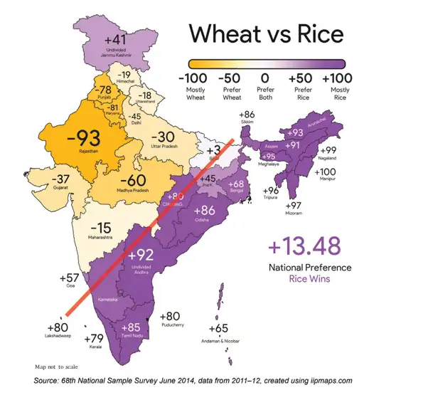
The mapped value represents the difference between per-capita rice and wheat consumption: positive values indicate greater rice preference, negative values greater wheat preference, and values near zero a more balanced preference. A value of +100 means the greatest rice-over-wheat difference on the scale, not that wheat is not consumed.
The sign indicates which grain is preferred; the map displays this difference on a scale from −100 to +100.
How to interpret a colour-coded map
- Read the colour key and identify what the two ends and the middle of the scale mean.
- Locate a state and match its shade to the scale.
- Compare shades across states to identify strongest preferences and near-balanced cases.
- Describe visible geographic patterns, such as the broad rice–wheat split marked by the red line.
What does a mapped value of −35 tell us about a state's rice and wheat preference?
- A state has a mapped value of −35. Since it is negative, wheat consumption per person is greater than rice consumption per person.
- The value shows a wheat preference, but it does not mean rice is not consumed.
Do not interpret +100 as zero wheat consumption. It indicates the highest rice-over-wheat difference on the displayed scale.
What a Strip Can Say
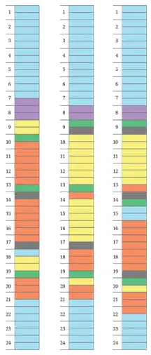
Multiply the number of boxes by the time represented by each box.
How to read a daily activity strip
- Identify the colour key for the activities.
- Use the time scale to find when each coloured section starts and ends.
- Count boxes and multiply by 30 minutes to find an activity’s duration.
- Compare strips to spot differences in routines and make reasonable inferences.
How long does an activity last if it fills 8 boxes?
- Suppose one activity occupies 8 consecutive boxes. Multiply the number of boxes by 30 minutes per box.
- Convert 240 minutes into hours.
A state is shown close to zero on the rice–wheat preference scale. What can you conclude?
A coloured activity section covers 6 boxes on Manoj’s strip. How much time does it represent?
Quick recap
- An infographic uses visuals and a key to communicate information and patterns.
- On the rice–wheat map, positive values favour rice, negative values favour wheat, and near-zero values are more balanced.
- A value of +100 indicates the greatest rice-over-wheat difference on the scale, not zero wheat consumption.
- Manoj’s strip has 48 boxes covering a full day, with 30 minutes represented by each box.
- Count the boxes in a coloured section and multiply by 30 minutes to find its duration.
- Comparing daily strips can reveal differences in routines, study, sleep, and free time.
Visualizing and Interpreting Data – Sleepy Deepy
Reading and Choosing Line Graphs
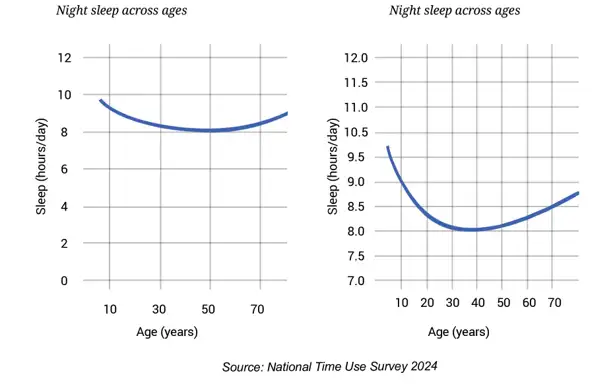
How to interpret a line graph
- Read the axis labels and units first.
- Check the scale and locate the required year, age or category.
- Read the corresponding value, estimating between grid lines only when needed.
- Describe increases, decreases, peaks, low points and comparisons using the graph.
- Do not infer causes or details that the graph does not show.
Mean and Median
Use for numerical data; is the number of values.
If the original mean is for values and new values have sum , use this to calculate the new mean.
Will the class mean height increase, decrease or stay the same?
- A class has mean height cm. Two new students have heights cm and cm. Let the original class size be .
- Compare the mean of the two new heights with the old class mean.
- The new class mean is greater than the old mean because the added students' mean is higher.
The mean of multiples of a number is not necessarily a multiple of that number. For example, the mean of two even numbers can be odd, and the mean of multiples of need not be a multiple of .
Do not assume that adding data automatically increases the mean. The direction of change depends on whether the added values' mean is above or below the original mean. Extra values alone do not determine the change in median.
Comparing and Questioning Graphs
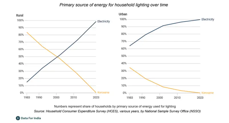
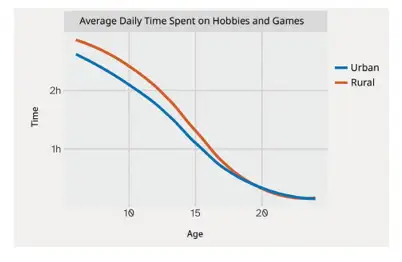
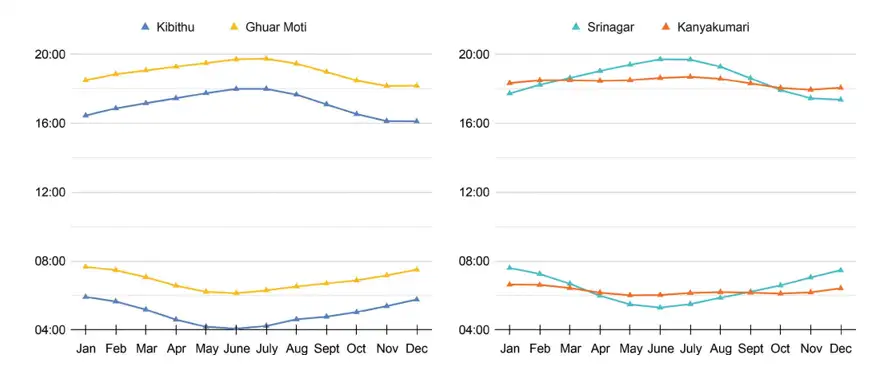
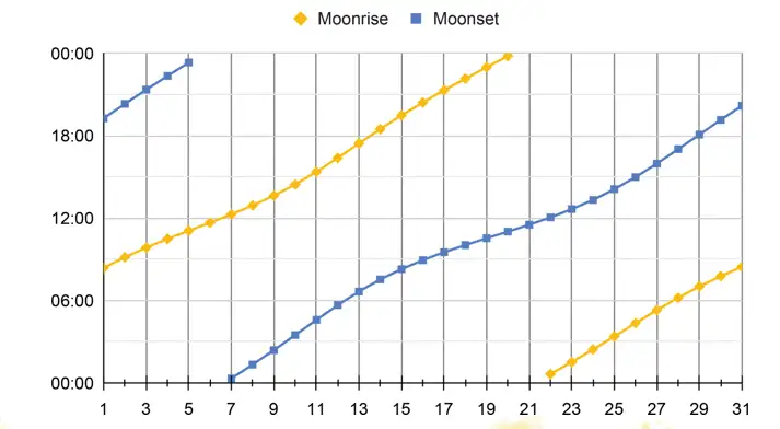
Plotting data as a line graph
- Choose an appropriate horizontal axis for the ordered values, such as years, and a vertical axis for the measured quantity.
- Select a consistent scale that fits the full range of values.
- Plot each value at its correct position and connect successive points in order.
- Label both axes, include units and add a clear title; use separate lines and a key when comparing groups.
From 2016 to 2025, which listed state had the greatest increase in iodised salt price?
Three people have weights that change by kg, kg and kg. What happens to the mean weight of the same group?
Is the mean of any five multiples of necessarily a multiple of ?
Quick recap
- Line graphs show how ordered data changes and are especially useful for many closely spaced values.
- Read carefully: Check axes, units and scale before describing a trend or comparing lines.
- Mean equals the sum of the values divided by their count.
- Adding values: The mean rises, falls or stays fixed according to how the added values' mean compares with the original mean.
- Median is found by ordering the data; with an even count, average the two middle values.
- Inference: A graph supports only conclusions that its displayed data can justify.
Summary
Mean as a Fair Share
Use this to find the fair share of a set of values.
For the values 2, 4, 6, and 8, find the mean and check the balance property.
- Find the mean of the values and compare the total distances on each side.
- Calculate the mean.
- Add the distances below and above the mean.
How Added Values Affect the Mean and Median
Add the new value to the original total, then divide by the updated number of values.
How do adding a value above or below the original mean affect the mean and median of 2, 4, and 6?
- Start with the values 2, 4, and 6; their mean and median are both 4.
- Add 10, which is above the mean; calculate the new mean and median.
- Add 0 instead; calculate the new mean and median.
Line Graphs and Exploring Data
Read a Line Graph
- Identify what each axis represents.
- Read the value at each time point.
- Follow the line to describe the trend and suggest a question for further investigation.
Describe the temperature trend and give a question the data could lead you to investigate.
- A line graph records temperatures of 20, 22, and 21 degrees on Monday, Tuesday, and Wednesday.
- Compare each consecutive value to describe the trend.
- Ask a follow-up question suggested by the data.
The mean of 3, 5, and 7 is 5. Check whether the total distances below and above the mean are equal.
A line graph shows a value of 12 on day 1, 15 on day 2, and 15 on day 3. Describe the change and suggest one question to investigate.
- The mean is the fair share and balances the total distances on its two sides.
- Adding a value above or below the mean moves the mean up or down; the median may respond differently.
- Line graphs make change over time visible, and data can prompt further questions.
Quick recap
- The mean is the total divided equally among all values.
- Distances below and above the mean have equal totals.
- Adding a value above the mean raises it; adding one below lowers it.
- The median can shift towards an added value or remain unchanged.
- A line graph shows how a quantity changes over time.
- Data patterns can lead to new questions for investigation.
Formula sheet
Mathematics — ALL CHAPTERS
1
A Square And A Cube
2
Power Play
3
A Story of Numbers
4
Quadrilaterals
5
Number Play
6
We Distribute, Yet Things Multiply
7
Proportional Reasoning-1
1
Fractions in Disguise
2
The Baudhayana-Pythagoras Theorem
3
Proportional Reasoning-2
4
Exploring Some Geometric Themes
5
Tales by Dots and Lines
6
Algebra Play
7
Area