Class 9 . Science . Exploration . Describing Motion Around Us
Chapter 4: Describing Motion Around Us
Ch 4
Science
Class 9
Motion in a Straight Line part 1
Studying Motion
- Motion is widespread: Objects ranging from astronomical bodies to tiny particles are in motion.
- Simplifying motion: Complex motion is first studied in idealised forms, including linear, circular and oscillatory motion.
- Chapter focus: The chapter develops the study of linear motion and uniform circular motion.
- Describing motion: Motion can be represented with words, measurements, equations and graphs; later topics include displacement, average velocity and average acceleration.
Motion in a Straight Line
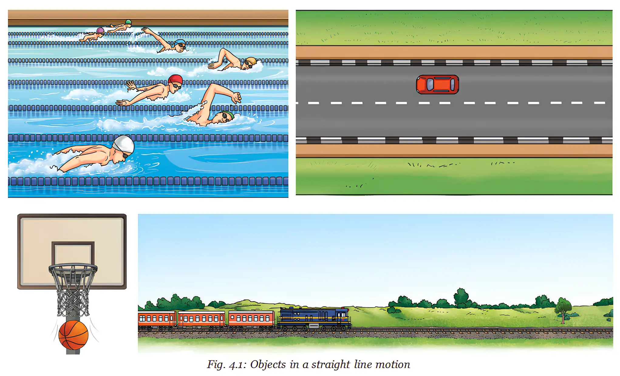
Linear motion — Motion of an object along a straight line; it is one of the simplest kinds of motion.
Examples
- Examples: Swimmers racing in a straight lane, a vertically falling ball, a car on a straight road and a train on a straight track.
Describing Position
Position — The location of an object at a particular time, described by its distance and direction from a fixed reference point.
Reference Point and Direction
- Reference point: Choose a fixed point from which the object's location is measured.
- Position needs direction: Distance alone is not enough; also state the direction from the reference point.
- Straight-line convention: Mark the reference point as origin . Positions to its right are generally positive (), and positions to its left are negative ().
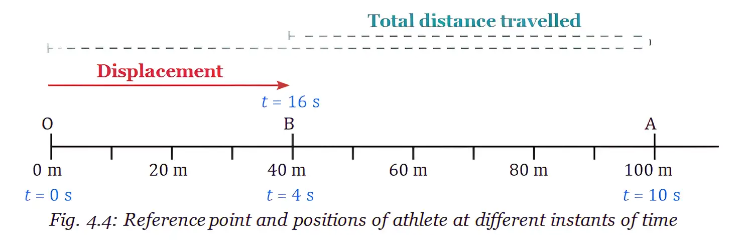
- Example: With as the reference point, the athlete's positions shown are and .

Motion — An object is in motion if its position relative to a reference point changes with time.
Rest — An object is at rest if its position relative to a reference point does not change with time.
| Point | Instant of time | Time interval |
|---|---|---|
| Meaning | A single clock reading at a particular time. | The duration between two instants, or two clock readings. |
Do not confuse an instant (one time reading) with a time interval (time elapsed between two readings).
Quick recap
- Linear motion is motion along a straight line.
- The chapter also studies uniform circular motion alongside linear motion.
- Describe position using distance and direction from a fixed reference point.
- In the usual number-line convention, right is positive and left is negative.
- Motion means position changes relative to a reference point; rest means it does not.
- An instant is one clock reading; an interval is the duration between two readings.
Motion in a Straight Line part 2
Distance Travelled and Displacement
Distance travelled — The total length of the path covered by an object; it has magnitude only.
Displacement — The net change in an object's position between two instants, including its direction.
| Point | Distance travelled | Displacement |
|---|---|---|
| What it measures | Entire path covered | Change from initial to final position |
| Direction needed? | No | Yes; from the initial position towards the final position |
| Magnitude | Length of the path | Separation between initial and final positions |
| SI unit | Metre () | Metre () |
Scalars, vectors and magnitude
- Scalar: A physical quantity specified by its numerical value and unit only; distance is a scalar.
- Vector: A physical quantity described by magnitude and direction; displacement is a vector.
- Magnitude: The numerical value of a quantity, expressed with its unit.
The sign indicates direction relative to the chosen positive direction.
Athlete example
- Route: The athlete runs from to (), then back to ; .
- Distance: .
- Displacement: The final position is from , so displacement is in the positive direction.
How Distance and Displacement Are Related
The magnitude of displacement cannot exceed the total distance travelled.
When are they equal?
- Same direction: For straight-line motion without turning back, distance travelled equals the magnitude of displacement.
- Returning to the start: Displacement is zero, while distance travelled is the length of the route covered and is not zero.
Vertical Motion and Return to the Start
Ball thrown vertically upward
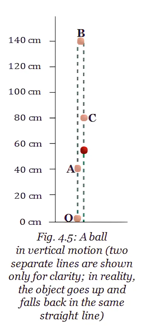
- Path: The ball moves upward and then falls back along the same vertical straight line; this is straight-line motion, even though its direction reverses.
- At position : The ball has travelled and its displacement from is upward.
- On the way down: Distance continues to accumulate; displacement is measured from to the ball's current position.
- Back at : Displacement is zero. If the ball reaches a maximum height , its total distance for the complete up-and-down journey is .
Inclined Track and Position Representation
Interpreting the inclined-track example
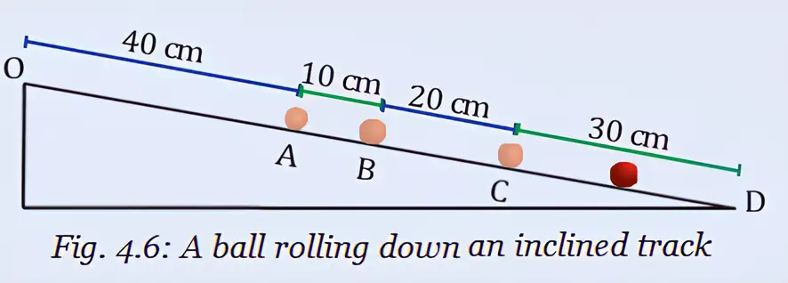
- Check the path: An inclined track is not necessarily a straight-line path; use the track's actual shape to decide whether the motion is straight.
- Position scale: A horizontal line may be used to mark positions along a chosen direction, but that representation alone does not prove the object's physical path is straight.
- Distance and displacement: They are equal in magnitude only when the object moves along a straight path in one direction without turning back.
When will the athlete's displacement be zero, and what distance will she have travelled if she returns to ?
Does vehicle fuel use depend on total distance travelled or displacement?
Do not confuse distance with displacement: distance includes the whole path, while displacement depends only on the initial and final positions and has a direction.
Quick recap
- Distance is the total path length; displacement is the directed change from start to finish.
- Both quantities have the SI unit metre (); distance is scalar and displacement is vector.
- The magnitude of displacement is always less than or equal to distance travelled.
- Distance equals displacement magnitude when straight-line motion continues in one direction without turning back.
- Returning to the starting point gives zero displacement, but the distance travelled is not zero.
- Vehicle fuel use is related to total distance travelled, not just displacement.
Motion in a Straight Line part 3
Average Speed and Types of Motion
Average speed — The total distance travelled divided by the time interval taken.
Here, is total distance and is the time interval.
- Direction: Distance has magnitude only, so average speed gives no direction.
- Uniform motion: In straight-line motion, equal distances are covered in equal time intervals, however the intervals are chosen; speed is constant.
- Non-uniform motion: Unequal distances are covered in equal time intervals; speed may increase, decrease, or both.
- Increasing speed: Increasing distances in successive equal time intervals indicate increasing speed.
| Motion type | Distance in equal time intervals | Speed |
|---|---|---|
| Uniform | Equal | Constant |
| Non-uniform | Unequal | May increase or decrease |
Meeting Motion Example
- Approach speed: Two postmen walking towards each other at and yojanas per day cover yojanas together each day.
- Meeting time: For a separation of yojanas, time is days. They cover and yojanas, respectively.
Average Velocity
Average velocity — The displacement divided by the time interval over which that displacement occurs.
Here, is displacement and is the time interval.
- Direction: Average velocity includes both magnitude and direction; for straight-line motion, its direction is the direction of displacement.
- Sign: Choose a positive direction; velocity in that direction is positive and velocity in the opposite direction is negative.
- Units: Average speed and average velocity both use (or ); is also common.
- Rate of change: A change in a quantity divided by the corresponding time interval is its average rate of change. Average velocity is the average rate of change of position.
- For straight-line motion in one direction, average speed equals the magnitude of average velocity.
- If an object returns to its starting point, its displacement—and hence average velocity—is zero, even if it travelled a non-zero distance.
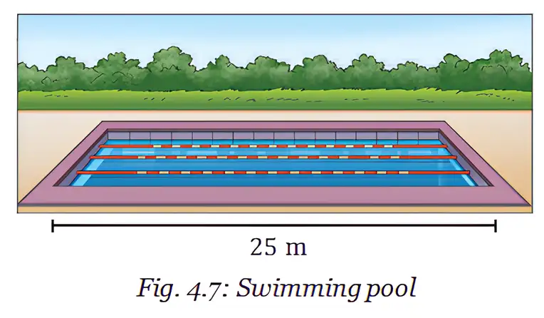
Swimming Pool Example
- Journey: Sarang swims to the other end of a pool and back in ; distance is and displacement is .
- Average speed: .
- Average velocity: .
A trip consists of north in , then south in . Find the average speed and average velocity.
Velocity at an Instant
- Instantaneous velocity: The velocity of an object at a particular instant; throughout this chapter, “velocity” refers to this unless stated otherwise.
- Average vs instantaneous: Average velocity over a long interval can differ from the velocity at a particular instant.
- Speedometer: A vehicle’s speedometer reading is nearly, but not exactly, the magnitude of its instantaneous velocity; the tyre direction indicates the velocity direction.
- Limit idea: As the time interval around an instant becomes infinitesimally small, average velocity approaches a fixed value called instantaneous velocity.
Quick recap
- Average speed = total distance divided by time; it has no direction.
- Uniform motion covers equal distances in equal time intervals; non-uniform motion does not.
- Average velocity = displacement divided by time and includes direction.
- Speed and velocity share SI units: ; is also used.
- Average speed equals the magnitude of average velocity when motion is in one direction.
- A round trip has zero displacement and average velocity, but can have non-zero average speed.
- Velocity at an instant is called instantaneous velocity.
Motion in a Straight Line part 4
Average Acceleration
Average acceleration — The change in an object's velocity divided by the time interval over which the change occurs.
Use when velocity changes from at time to at time . Its SI unit is or .
Direction and meaning
- Velocity change: Acceleration can result from a change in speed, direction, or both.
- Speed increasing: For straight-line motion, acceleration acts in the direction of velocity.
- Speed decreasing: Acceleration acts opposite to the direction of velocity.
- Constant velocity: An object may move fast yet have zero acceleration if its velocity is not changing.
| Motion | Direction of acceleration |
|---|---|
| Speed increasing | Same as velocity |
| Speed decreasing | Opposite to velocity |
Calculating Average Acceleration
Bus example
- Accelerating: The bus changes speed from to in .
- Braking: From , the bus stops in .
A negative acceleration does not necessarily mean the object is moving in the negative direction; here it indicates acceleration opposite to the bus's velocity.
Constant Acceleration and Free Fall
Constant acceleration — Acceleration is constant when velocity changes by equal amounts in equal time intervals throughout the motion.
Falling object example
- Velocity changes: A dropped object’s downward velocity increases by each successive second.
- Acceleration: Each one-second interval gives an average acceleration of , so the acceleration is constant.
- Name and direction: This downward acceleration is due to Earth's gravitational force and is denoted by .
Choose a positive direction and origin for a motion problem, then keep that choice unchanged throughout the solution.
Instantaneous Acceleration
Instantaneous acceleration — The acceleration of an object at a particular instant of time.
Quick recap
- Average acceleration is change in velocity divided by elapsed time.
- Its SI unit is , and its direction depends on the change in velocity.
- Speeding up in a straight line: acceleration is in the direction of velocity; slowing down: it is opposite.
- An object moving at constant velocity has zero acceleration, regardless of how fast it moves.
- Constant acceleration means equal velocity changes in equal time intervals; a falling object has acceleration downward.
- Choose a coordinate direction once and keep it fixed; instantaneous acceleration describes acceleration at an instant.
Graphical Representation of Motion part 1
Why Use Graphs for Motion?
Graphical representation of motion — A visual representation showing how quantities such as position, velocity or acceleration change with time.
- Uses: Motion graphs help compare objects, calculate physical quantities and identify uniform or non-uniform motion.
- Axes: A graph shows the dependence of one physical quantity on another, commonly position or velocity against time.
- Scope: Here, motion is along a straight line in one direction; distance equals displacement magnitude, and speed equals velocity magnitude.
- When starting at zero: The position–time graph matches the distance–time graph; the velocity–time graph matches the speed–time graph.
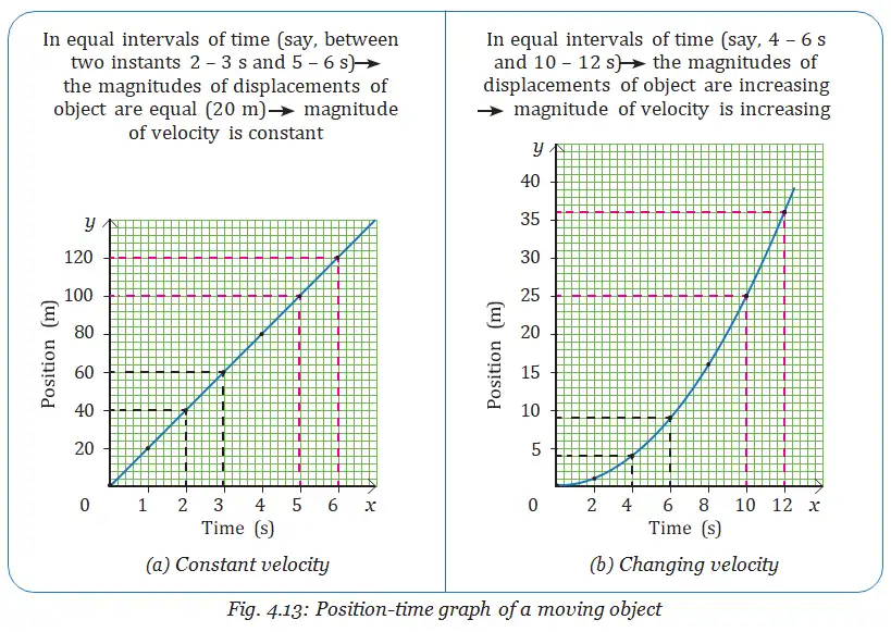
Plotting a Position–Time Graph
Graph basics
- Origin: The point where the two perpendicular axes meet is the origin, O.
- Axes: Time is placed on the horizontal x-axis and position on the vertical y-axis for a position–time graph.
- Scale: Choose a convenient scale for each axis that represents the data clearly and uses the available graph space.
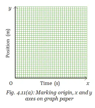
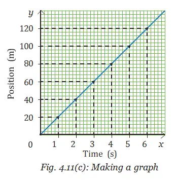
| Time | Position |
|---|---|
| 0 s | 0 m |
| 1 s | 20 m |
| 2 s | 40 m |
| 3 s | 60 m |
| 4 s | 80 m |
| 5 s | 100 m |
| 6 s | 120 m |
Plotting the graph
- Draw perpendicular axes, marking the horizontal axis as time and the vertical axis as position.
- Choose a suitable scale for each axis; for the example, use 5 divisions = 1 s on x and 5 divisions = 20 m on y.
- Mark the time and position values according to their scales.
- Plot each time–position pair; for example, the pair 1 s and 20 m is one plotted point.
- Join the plotted points to form the position–time graph.
Reading the plotted shape
- Straight line: The example’s points lie on a straight line, showing uniform motion.
- Intermediate points: Points between the given data values represent possible positions only if the vehicle keeps moving at constant speed.
- Graph meaning: A motion graph shows how position changes with time relative to the origin; it is not a map of the route taken.
Position–Time Graph for a Vehicle Speeding Up
| Time | Position |
|---|---|
| 0 s | 0 m |
| 2 s | 1 m |
| 4 s | 4 m |
| 6 s | 9 m |
| 8 s | 16 m |
| 10 s | 25 m |
| 12 s | 36 m |
- Scale for this data: Use 5 divisions = 2 s on the time axis and 5 divisions = 5 m on the position axis.
- Shape: The plotted points do not form a straight line; join them with a curve.
- Interpretation: This curved position–time graph represents a vehicle whose speed is increasing.
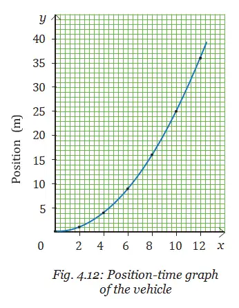
What does the shape of a position–time graph indicate in these examples?
Quick recap
- Motion graphs show how physical quantities change with time and help compare motion.
- For a position–time graph, plot time on the x-axis and position on the y-axis.
- Choose clear axis scales, plot each time–position pair and connect the points.
- A straight position–time line represents uniform motion; intermediate values assume constant speed.
- A graph describes position relative to the origin, not the route followed.
- A curved position–time graph can represent a vehicle speeding up.
Graphical Representation of Motion part 2
Position–Time Graphs
Position–time graph — A graph that shows how an object's position changes with time.
Reading the graph
- Position: Read the object's position at any instant from the graph.
- Straight sloping line: Position changes uniformly with time, so the object moves with constant velocity.
- Curved line: The rate of change of position is not constant; the object is in accelerated motion.
Velocity from the Slope
Slope of a graph — The change in the quantity on the vertical axis divided by the change in the quantity on the horizontal axis.
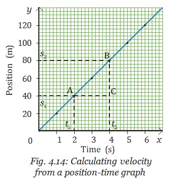
Finding average velocity
- Choose two points: Read their positions , and times , from the graph.
- Calculate: Average velocity magnitude equals change in position divided by the time interval.
- Geometry: This ratio is the slope of the line joining the two points; a steeper line means a greater velocity magnitude.
- Curved graph: The velocity at an instant can also be found geometrically, but this is studied in higher grades.
Use the positions and times at the two chosen points.
Example
- Given: Position changes from to between and .
- Calculation: .
Stationary Objects and Comparing Velocities
Special graph patterns
- Horizontal line: Position remains unchanged as time passes, so the object is stationary.
- Example: A horizontal line at means the vehicle is at rest from the origin.
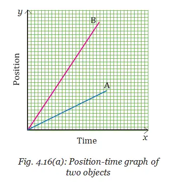
- Compare slopes: For the same time interval, the object with the steeper position–time line has the greater average velocity magnitude.
- Objects A and B: Over the same time interval, B has greater displacement and a steeper graph than A; therefore, B has the greater magnitude of average velocity.
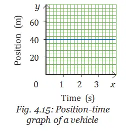
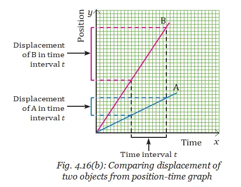
Do not confuse a position–time graph with a distance–time graph: a horizontal position–time line means the object's position is unchanged, so it is at rest.
What does the slope of a position–time graph represent?
What does a horizontal line on a position–time graph indicate?
Which object, A or B, has the greater magnitude of average velocity in the given graphs?
Quick recap
- A position–time graph gives an object's position at each instant.
- A straight sloping line indicates constant velocity; a curved line indicates changing velocity and accelerated motion.
- The slope of a position–time graph gives the rate of change of position.
- Average velocity magnitude is between two points.
- A steeper line over the same time interval indicates greater average velocity magnitude; object B's is greater than object A's in the given comparison.
- A horizontal position–time line means the object is at rest.
Velocity-time graphs
Describing motion
Position — An object's position is its location and direction relative to a reference point at a given instant.
Motion — An object is in motion if its position relative to a reference point changes with time.
Displacement — Displacement is the net change in an object's position between two instants.
Average speed — Average speed is the total distance travelled divided by the time interval.
Use total distance travelled over the time interval.
Average velocity — Average velocity is the displacement divided by the time interval in which the displacement occurs.
Use displacement over the time interval.
Reading velocity–time graphs
Velocity–time graph — A graph showing how an object's velocity changes with time.
Examples and graph shapes
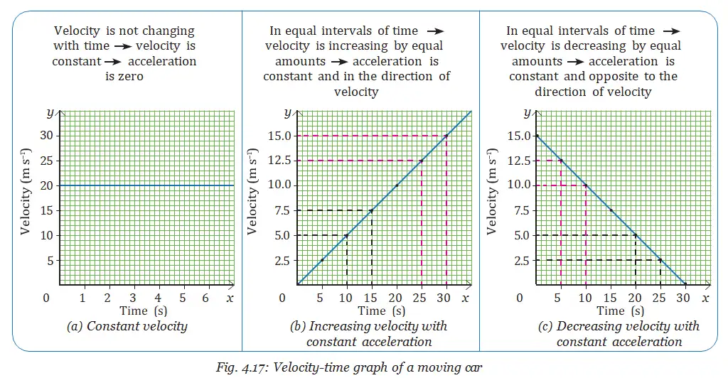
- Constant velocity: A car travelling at has a horizontal velocity–time graph.
- Increasing velocity: A straight rising line represents velocity increasing at a constant rate.
- Decreasing velocity: A straight falling line represents velocity decreasing at a constant rate; acceleration is opposite to the velocity direction.
| Time | Increasing velocity | Decreasing velocity |
|---|---|---|
Slope and area of a velocity–time graph
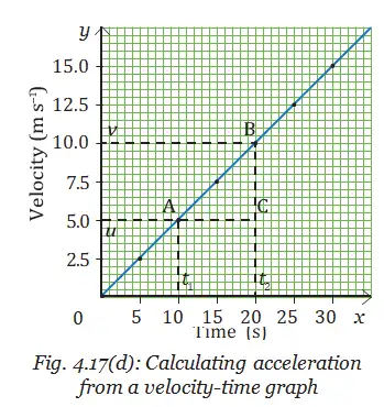
Slope — The slope of a velocity–time graph gives the acceleration.
For velocities and at times and , respectively.
Acceleration examples
- Constant velocity: The graph is horizontal, so its slope and acceleration are zero.
- Between and : Velocity rises from to , giving .
- Decreasing velocity: The same rate of decrease gives ; the negative sign indicates acceleration opposite to the velocity direction.
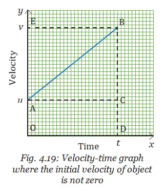
Area under the graph — The area between a velocity–time graph and the time axis over an interval gives the displacement during that interval.
The graph area is a rectangle.
Area examples
- Constant velocity: At for , displacement is .
- Increasing velocity: From to , area equals rectangle plus triangle: .
Kinematic equations for constant acceleration
Symbols and conditions
- Symbols: is initial velocity, is final velocity after time , is acceleration, and is displacement.
- Validity: These equations apply to straight-line motion with constant acceleration.
- Motion in one direction: Distance travelled equals the magnitude of displacement; speed equals the magnitude of velocity.
- Motion in both directions: Use the signs of , , and to show their directions.
Applying the kinematic equations
Braking and stopping distance
- Given: Braking acceleration is and final velocity is .
- Convert speeds: ; .
- Apply: From , the stopping distance is .
- Results: Stopping distances are from and from .
Safe following distance
- Vehicle speed, road surface, braking capacity and driver reaction time affect stopping distance.
- A longer stopping distance requires more space to stop safely.
- Maintain a safe gap and adjust it to the vehicle's speed and conditions; vehicle-to-vehicle (V2V) communication can warn of possible collisions.
Motion in a plane
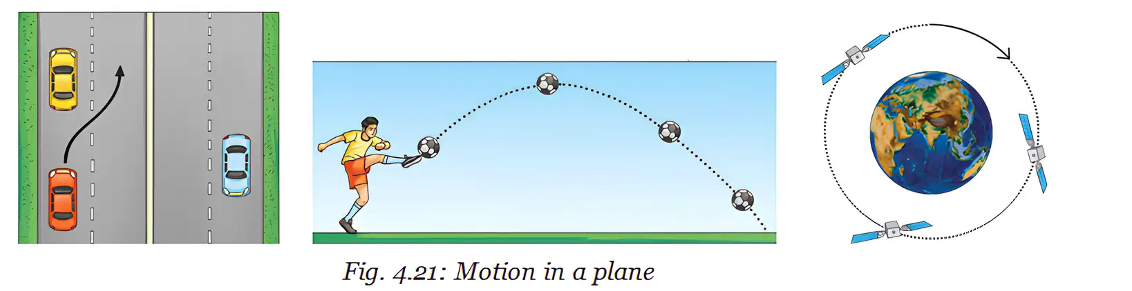
Motion in two dimensions — Motion in a plane, such as movement along a curved path or changing direction on a flat surface, is motion in two dimensions.
Examples
- Two dimensions: A vehicle overtaking another, a kicked ball following a curved path, and a satellite moving in a circular path.
- Three dimensions: Motion through space, such as a car climbing a mountain road, a bird flying or an aircraft moving through air.
Circular and uniform circular motion
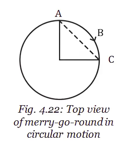
Circular motion — Motion along a circular path is called circular motion.
One revolution
- Distance: In one complete revolution on a circle of radius , distance travelled is the circumference, .
- Displacement: It is zero after one revolution because the object returns to its starting point.
If one revolution takes time .
Uniform circular motion
- Definition: Motion around a circular path at constant speed is uniform circular motion.
- Average velocity: Over a complete revolution, average velocity is zero because displacement is zero.
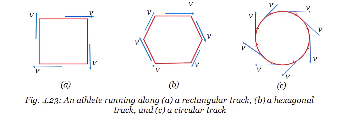
- Velocity: Speed is constant, but velocity changes continuously because its direction changes.
- Acceleration: Uniform circular motion is accelerated motion because a change in velocity direction is a change in velocity.
Direction of motion
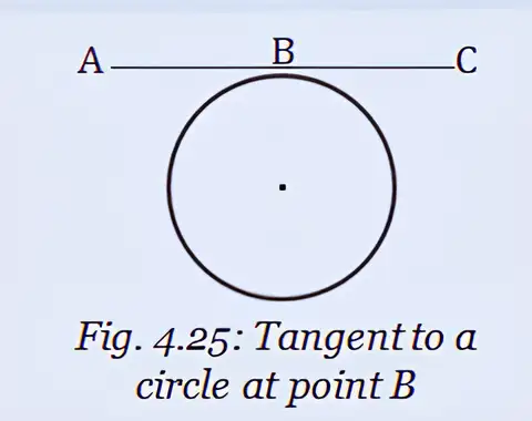
- Instantaneous velocity: At any point on a circle, velocity is along the tangent in the direction of motion.
- Release: If the circular constraint is removed, the object continues in a straight line in the direction it was moving at that instant.
- Ideal model: Perfect circular motion at constant speed is an idealisation, useful for understanding situations such as planetary orbits and vehicles turning.
Tangent — A straight line that meets a circle at exactly one point is a tangent to the circle at that point.
Acceleration does not require a change in speed: a change in velocity direction alone, as in uniform circular motion, also means acceleration.
What do the slope and area under a velocity–time graph represent?
When are the kinematic equations valid, and what are the three equations?
Why is uniform circular motion accelerated even when speed is constant?
Quick recap
- Position is measured relative to a reference point; motion means position changes with time.
- Average speed is total distance divided by time; average velocity is displacement divided by time.
- A velocity–time graph's slope gives acceleration and its area over an interval gives displacement.
- For straight-line motion with constant acceleration: , , and .
- Stopping distance depends on speed, road surface, braking capacity and reaction time; maintain a safe following gap.
- One circular revolution covers distance , has zero displacement, and takes time at average speed .
- Uniform circular motion has constant speed but changing velocity direction, so it is accelerated motion; instantaneous velocity follows the tangent.
Science — ALL CHAPTERS
1
Exploration: Entering the World of Secondary Science
2
Cell: The Building Block of Life
3
Tissues in Action
4
Describing Motion Around Us
5
Exploring Mixtures and their Separation
6
How Forces Affect Motion
7
Work, Energy, and Simple Machines
8
Journey Inside the Atom
9
Atomic Foundations of Matter
10
Sound Waves: Characteristics and Applications
11
Reproduction: How Life Continues
12
Patterns in Life: Diversity and Classification
13
Earth as a System: Energy, Matter, and Life