Class 7 . Mathematics . Ganita Prakash Part II . Connecting the Dots
Chapter 5: Connecting the Dots
Ch 5
Mathematics
Class 7
Of Question and Statements
Statistical Thinking and Statements
Statistical thinking
- Statistical thinking uses data and patterns to make reasonable estimates or predictions, while recognising that conclusions may not be certain.
- Example: If one person is 5 feet tall and another is 6 feet tall, height alone cannot tell us their genders; any guess is only a general expectation.
Statistical statement — A claim or summary about a phenomenon expressed using numerical values, proportions, probabilities, or predictions.
Examples of statistical statements
- Prediction: A batter’s consistent performance may suggest that she could score a century in the next match.
- Estimate: A person takes about 15 minutes to cycle home from school.
- Change: A village’s population has fallen by about 100 over a decade.
- Association: Eating more fruit and vegetables has coincided with being able to run farther each day.
- Routine: A student spends about 7 hours a day at school.
Statistical Questions
Statistical question — A question answered by collecting and analysing data that can vary across people, places, or times.
How to recognise one
- Variation: The answers are not all expected to be the same.
- Data needed: Many observations must be collected and examined to answer reliably.
- Conclusion: The analysis supports a summary or conclusion, rather than a single fixed answer.
- Examples: Heights of Grade 7 students; typical onion prices in two towns, which may vary over time.
Deciding whether a question is statistical
- Identify what information the question asks for.
- Check whether answers may vary across the people, places, or times involved.
- Decide whether collecting and analysing data is needed to give a useful answer.
| Question | Statistical? | Reason |
|---|---|---|
| What is the price of a tennis ball in India? | Yes, if comparing prices | Prices may vary across sellers and places, so multiple observations are useful. |
| How old are the dogs on this street? | Yes | Different dogs can have different ages. |
| What fraction of students in your class like walking up a hill? | Yes | A class survey collects varied responses. |
| Do you like reading? | No | As phrased, it asks one person for one answer. |
| Approximately how many bricks are in this wall? | No | It asks for one count of a particular wall. |
| Who was the best bowler in yesterday’s match? | No | It asks for one result from a particular match. |
| What was the rainfall pattern in Barmer last year? | Yes | Rainfall varies over time, so observations across the year are needed. |
Do not decide only from the wording. Ask whether the answer requires data with variation; a question about one fixed person, object, or event is usually not statistical.
Is “How tall are Grade 7 students in our school?” a statistical question?
- Decide whether “How tall are Grade 7 students in our school?” is statistical.
- Heights are expected to differ from student to student.
- Collecting and analysing the students’ heights gives a useful summary of the group.
Statistics
Statistics — The study of collecting, organising, analysing, interpreting, and presenting data.
What statistics involves
- Collect data
- Organise data
- Analyse data
- Interpret results
- Present findings
Is “How many hours do students in this class sleep each night?” a statistical question?
Is “What is the length of this ruler?” a statistical question?
Quick recap
- Statistical thinking uses observed patterns to make estimates or predictions, not guarantees.
- A statistical statement expresses a numerical claim, summary, proportion, probability, or prediction.
- A statistical question involves variation and is answered by collecting and analysing data.
- One fixed person, object, or event generally gives a non-statistical question.
- Statistics involves collecting, organising, analysing, interpreting, and presenting data.
Representative Values
Comparing Performance
| Player | Match 1 | Match 2 | Match 3 | Match 4 |
|---|---|---|---|---|
| Shubman | ||||
| Yashasvi |
Different Ways to Compare
- Highest score: Shubman's top score is , but one high score alone may not represent the whole performance.
- Total runs: Yashasvi scored runs, compared with Shubman's .
- Consistency: Compare the difference between the highest and lowest scores; a smaller difference can indicate more consistent scores.
Why Totals Can Mislead
| Player | Match 1 | Match 2 | Match 3 | Match 4 | Match 5 |
|---|---|---|---|---|---|
| Shubman | |||||
| Yashasvi | Did not play |
Compare Fairly
- Different numbers of matches: Shubman scored runs in matches; Yashasvi scored runs in matches.
- Better comparison: Compare runs per match rather than totals when the groups contain different numbers of values.
Average (Arithmetic Mean) — A representative value found by dividing the sum of all data values by the number of values.
The mean balances higher and lower values in a data group. It is useful for comparing groups of different sizes.
Add all the values and divide by the number of values.
Finding the Mean
- Add all the values in the data group.
- Count the number of values.
- Divide the total by the count.
Who had the higher average number of runs per match?
- Find the mean runs per match for each player in the second series.
- Divide Shubman's total by the five matches he played.
- Divide Yashasvi's total by the four matches he played.
Do not compare totals alone when the groups have different sizes; divide each total by its number of values. Also, , not .
A player scores , , and runs. Find the mean score.
Team A scores , , and runs. Team B scores and . Which team has the higher mean?
Quick recap
- A representative value summarises a group of data.
- The arithmetic mean is the sum of values divided by their count.
- The mean balances high and low values in a data group.
- Use the mean to compare groups with different numbers of values.
- In the second series, Yashasvi's mean is runs and Shubman's is runs.
Average as Fair-Share
Average as an Equal Share
Average (arithmetic mean) — The average is the equal share each value would receive if the total were shared evenly among all values.
Understanding the Average
- Fair share: Add all values, then divide the total by the number of values.
- Equalising value: The average represents a collection by balancing its values.
- Flowers: For daily counts , the average is flowers per day—as if the same number bloomed each day.
If a total of is shared equally among values, each share is the arithmetic mean, .
Use this to find the equal share or representative value of a data set.
Finding an Average
- Add all the data values to find the total.
- Count the number of values.
- Divide the total by the number of values.
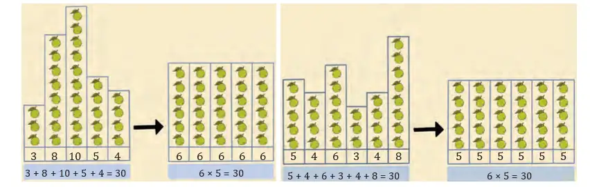
Which group gets the larger equal share of guavas?
- Shreyas’s group has members and collected guavas.
- Parag’s group has members and collected guavas.
Comparing Data and Using Dot Plots
Dot plot — A dot plot places each data value as a dot on a number line to show frequencies, clusters and spread.
Comparing Data
- Useful measures: Compare the minimum, maximum, average, total and range of a data set.
- Range: It measures the distance between the maximum and minimum values.
- Dot-plot reading: Dots are ordered by value; stacked dots show repeated values. Equal spacing represents equal intervals on both axes.
- Strength: A dot plot makes clusters, spread and extreme values easy to notice; Wahapur’s onion prices are more spread out than Yahapur’s.
- Limitation: Sorting the values removes their original order, so a dot plot cannot show which price belonged to which month.
- Grouping: Between and , Wahapur has prices and Yahapur has none.
| Month | Yahapur | Wahapur |
|---|---|---|
| January | ||
| February | ||
| March | ||
| April | ||
| May | ||
| June | ||
| July | ||
| August | ||
| September | ||
| October | ||
| November | ||
| December |
The range describes the spread from the smallest to the largest value.
Comparing Two Data Sets
- Find the total and average of each set using the same number of values.
- Find each set’s minimum, maximum and range.
- Compare the measures that match the question; one measure alone may not describe the whole data set.
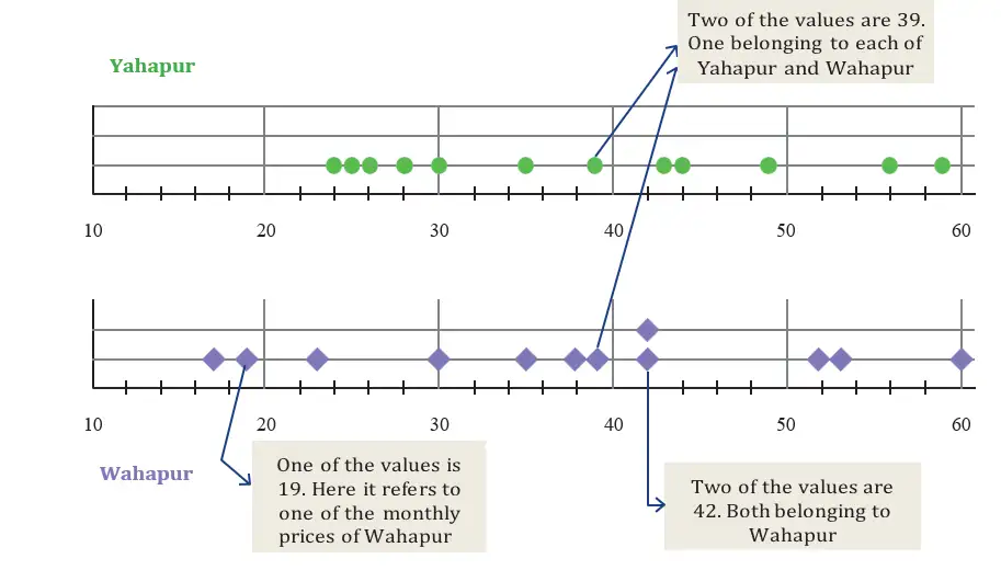
Which town has the higher average onion price, and which town’s prices have the greater range?
- Yahapur’s yearly total is across months; its minimum is and maximum is .
- Wahapur’s yearly total is across months; its minimum is and maximum is .
- Compare the averages and ranges.
Other Ways to Compare the Onion Prices
- Monthly comparison: Yahapur’s price is higher in months, Wahapur’s in months, and they are equal in month.
- Totals: Yahapur’s total is , while Wahapur’s is ; a total alone does not show how prices vary through the year.
- Interpretation: Compare several relevant features rather than relying only on the highest price or another single measure.
Shreyas made bounces in attempts. Find his average number of bounces.
Nikhil’s 100 m race times were seconds. Sunil’s were seconds. Who ran quicker on average?
A school’s enrolment over six years was . Find the mean enrolment.
Quick recap
- Average = total of values divided by the number of values; it represents an equal share.
- Find an average by adding the values, counting them and dividing the total by the count.
- Range = maximum minus minimum; it measures the distance between the extremes.
- Dot plots show ordered values, frequencies, clusters, spread and extreme values.
- A dot plot can lose original order, so it cannot preserve month-by-month pairings.
- The onion-price dot plot uses a horizontal scale from to .
- Compare data using relevant measures such as average, total, range and value-by-value comparisons.
Averages Around Us
Arithmetic Mean
Use for any data set with values.
Finding the Mean
- Add all the data values.
- Divide the total by the number of values.
What is the mean number of newspaper pages per day?
- The newspaper has these page counts from Monday to Sunday.
- Add the seven values.
- Divide by the number of days.
Median
Arrange values in ascending order; denotes the value at position .
Arrange values in ascending order; denotes the value at position .
Finding the Median
- Arrange the values from smallest to largest.
- For an odd count, select the middle value.
- For an even count, average the two middle values.
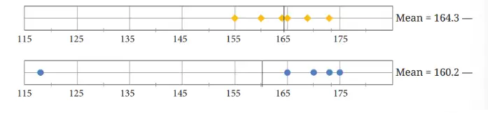
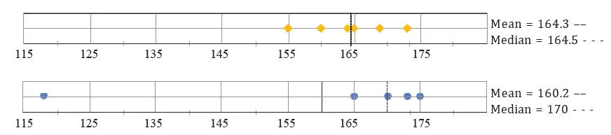
Find the median heights of Poovizhi's and Yaangba's families.
- Sort Poovizhi's family heights; there are five values, so select the third.
- For Yaangba's family, sort the six heights and average the third and fourth.
- Calculate the even-set median.
Outliers and Choosing a Representative
| Point | Mean | Median |
|---|---|---|
| How it is found | Total of values divided by their count | Middle value after arranging the data |
| Effect of an outlier | Can shift substantially | Usually changes less |
| Useful when | Data is reasonably balanced | Data contains extreme values |
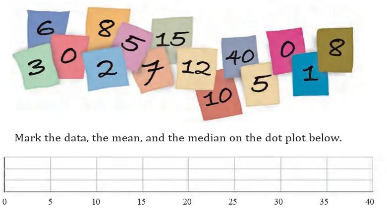
Mean and Median in the Newspaper Data
- Ordered pages: .
- Median: The middle value is pages; the mean is about pages, so they are close.
How Outliers Affect the Mean and Median
- Outlier below the data: The mean may become less than the median.
- Outlier above the data: The mean may become greater than the median.
- Outliers on both sides: Their effects on the mean can partly offset, while the median is generally still less sensitive to their distance from the centre.
Measures of central tendency — The mean and median are measures of central tendency: they describe the centre around which data values tend to gather.
Find the mean and median of .
Find the mean and median of . Which better represents most values?
Find the median of .
Do not find the median before sorting the data. With an even number of values, average the two middle values instead of choosing just one.
Quick recap
- Mean = total of the values divided by their count.
- Find the median by sorting the data and selecting the middle value.
- For an even-sized data set, the median is the average of the two middle values.
- An outlier is a value that differs significantly from most of the data.
- Outliers can pull the mean towards themselves; the median is usually less affected.
- Mean and median are measures of central tendency that describe the centre of data.
Of Ends and The Essence
Spread and centre in data
Variability — Variability describes how spread out the data values are, especially between the minimum and maximum.
Ways to describe data
- Range is the difference between the greatest and least values; it gives a quick measure of spread.
- Mean and median describe the centre of data, but they can give different perspectives.
- Dot plots show clusters, gaps, spread and the centre; compare them with the mean and median.
Mean — The mean is the sum of all data values divided by the number of values.
Median — The median is the middle value after arranging data in order; with an even number of values, it is the mean of the two middle values.
For any non-empty data set, the mean and median lie between its minimum and maximum. A mean below the median can indicate that lower values are pulling the mean down.
Arrange the data in increasing order before finding the median.
Describe a data set
- Find the minimum and maximum, then calculate the range.
- Find the mean and median to describe the centre.
- Use the dot plot to compare centres and spreads; do not assume every value follows the group average.
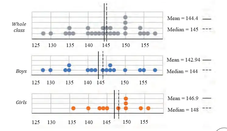
Compare the spread and centre of the class heights, and find how many students and boys are taller than the class mean.
- There are 17 boys and 11 girls; their total heights are 2,430 cm and 1,616 cm.
- The boys' heights range from 128 cm to 158 cm; the girls' range from 136 cm to 156 cm.
- Boys' mean and median are 142.94 cm and 144 cm; girls' are 146.9 cm and 148 cm. The class median is 145 cm.
- Eight boys and seven girls are taller than the class mean.
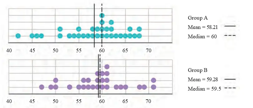
Comparing estimates of one minute
Compare the two groups
- Centre: Compare means and medians to see which group's estimates are closer to 60 seconds overall.
- Variability: A group whose estimates span a wider interval is less consistent.
- Dot plots: Compare each group's typical estimate, spread, clusters and unusually high or low values.
Zero and missing data
Zero value — Zero is a recorded value: it means the measured quantity was none.
Missing value — A missing value means no measurement or observation is available; it is not the same as zero.
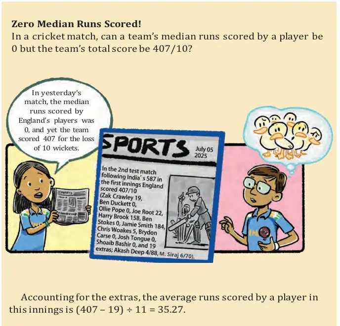
Include recorded zeroes when they belong to the question being studied; exclude missing values. Choose a time period that matches the question: for example, use fruiting-season months for average mango yield during that season, but all months for an annual monthly average.
Find the mean and median runs per match played for the scores 57, 13, 0, 84, —, 51, 27.
- The player scored 57, 13, 0, 84, 51 and 27 in six matches played; the dash means the player did not play that match.
- Include the zero score, but do not include the unplayed match in the total or divisor.
- Arrange the six scores and average the two middle values to find the median.
Applying the ideas
For daily water usages of 5.6, 8, 3.09, 12.9, 6.5, 12.1, 11.3, 20.5 and 7.4 litres, can the mean or median be between 25 and 30 litres?
For the domestic-animal counts 0, 1, 0, 4, 8, 0, 0, 2, 1, 1, 5, 3, 4, 0, 0, —, 10, 25, 2, —, 2, 4, find the mean and median and describe the data.
Sumo wrestler weights are 295.2, 250.7, 234.1, 221.0 and 200.9 kg; ballet dancer weights are 40.3, 37.6, 38.8, 45.5, 44.1 and 48.2 kg. Approximately how many times heavier is a sumo wrestler?
Quick recap
- Variability describes spread; range = maximum − minimum.
- Use mean and median together to describe the centre of data.
- Dot plots show spread, clusters, gaps and possible unusual values.
- Mean and median lie between the minimum and maximum data values.
- A recorded zero is included; a missing value is excluded from calculations.
- Choose observations and time periods that match the question.
Visualising Data
Data visualisation — Presenting data visually, such as with graphs, so that patterns and comparisons are easier to understand.
Grouped column graphs
Clustered column graph — A graph that places columns for two or more data groups side by side for each category; with two columns per group, it is also called a double column graph.
| Location | Jan | Feb | Mar | Apr | May | Jun | Jul | Aug | Sep | Oct | Nov | Dec |
|---|---|---|---|---|---|---|---|---|---|---|---|---|
| Yahapur | 25 | 24 | 26 | 28 | 30 | 35 | 39 | 43 | 49 | 56 | 59 | 44 |
| Wahapur | 19 | 17 | 23 | 30 | 38 | 35 | 42 | 39 | 53 | 60 | 52 | 42 |
How to read a grouped graph
- Clusters: Each month has two adjacent columns, one for each location.
- Comparison: Compare column heights within a cluster to see which location had the higher price and estimate the difference.
- Scale: Read the vertical-axis markings before estimating values or differences.
- Accessibility: Colours, dots, and slanted patterns can distinguish groups, including in greyscale or for readers who have difficulty distinguishing colours.
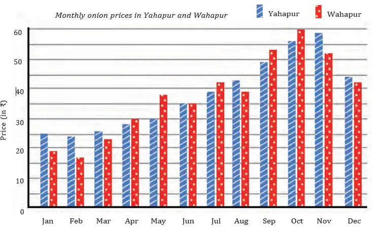
Use the axis scale to convert a bar's length into the value it represents. Here, is the data value, is the graph length, and is the value per unit length.
Compare two columns
- Find the category and read the two values using the graph scale.
- Subtract the smaller value from the larger to find the difference.
- State which group has the larger value and give the difference.
Which location had the higher onion price in January, and by how much?
- In January, compare the onion prices in Yahapur and Wahapur.
- Subtract the smaller price from the larger.
- Yahapur's price was higher by 6.
Do not compare bar heights without checking the axis scale; equal lengths represent equal values only when the same scale is used.
Reading and interpreting a multi-bar graph
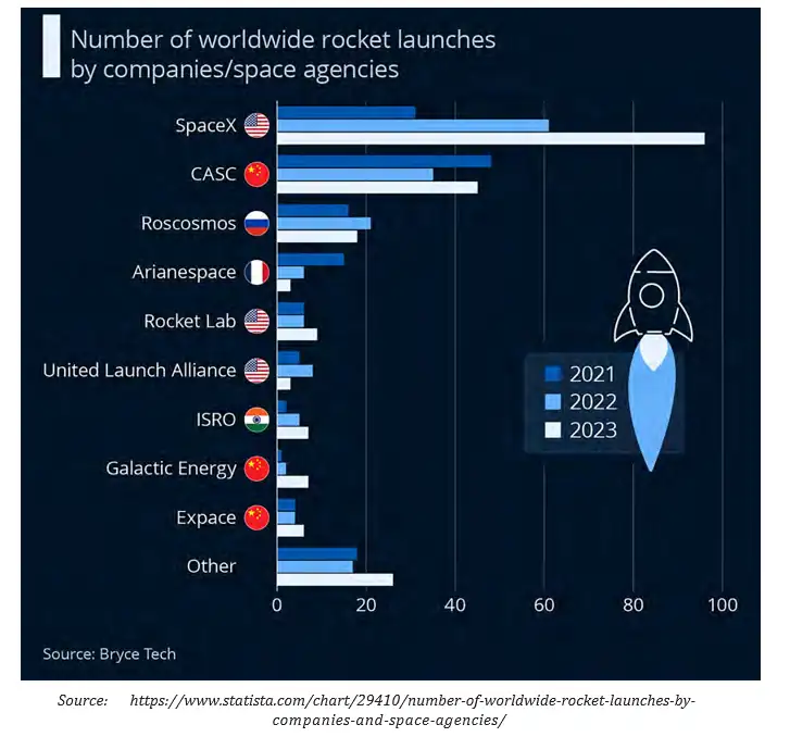
Two steps for interpreting a graph
- Identify what is shown: categories, time periods, scale, arrangement, and visible patterns.
- Infer what the graph supports: compare values, describe trends, and check claims against the data.
Rocket-launch graph: identify the information
- Bars: Three adjacent bars show each organisation's launches in 2021, 2022, and 2023.
- Scale: One unit of bar length represents 20 rockets; use the horizontal-axis markings to estimate counts.
- Others: This category combines multiple organisations to keep the graph concise.
- Ordering: Months are ordered to show change across the year; changing the order of organisations does not change the data's meaning.
A trend is found by comparing an organisation's values across years. A claim about a total or an average must use all relevant values, not just one bar.
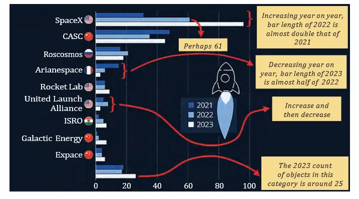
Rocket-launch graph: conclusions stated from the data
- Leading countries: The USA, China, and Russia were the leading rocket-launching countries in the period shown.
- SpaceX: It launched about twice as many rockets in 2022 as in 2021, then about 35 more in 2023 than in 2022.
- Arianespace: Its launch count decreased each year.
- United Launch Alliance: It launched more in 2022 than in 2021, then fewer in 2023 than in either earlier year.
- Others: The combined category launched about 25 rockets in 2023.
For a claim about three-year totals, add all three bars; for an average, add the three values and divide by . A single year's bar cannot prove a multi-year claim.
In October, which town had the higher onion price, and what was the difference?
If a rocket-launch bar is 4 units long, about how many launches does it represent?
What trend is stated for Arianespace's launches across 2021–2023?
Quick recap
- Data visualisation presents information so patterns and comparisons are easier to see.
- A clustered or double column graph places the groups' bars side by side for each category.
- Read the axis scale before comparing bar heights or estimating values.
- Interpret a graph by identifying its categories, scale, and patterns, then drawing conclusions supported by the data.
- Use all relevant bars to check claims about totals, averages, or year-to-year trends.
Summary and Winter at the same time
Monthly Daylight Data
Daylight hours — The number of hours in a day when the Sun is at least partly above the horizon.
| City | Jan | Feb | Mar | Apr | May | Jun | Jul | Aug | Sep | Oct | Nov | Dec |
|---|---|---|---|---|---|---|---|---|---|---|---|---|
| City 1 | 210 | 257 | 372 | 441 | 536 | 564 | 555 | 465 | 394 | 310 | 222 | 186 |
| City 2 | 459 | 384 | 381 | 327 | 304 | 276 | 295 | 318 | 369 | 409 | 435 | 468 |
Here, is the month's total daylight hours and is the number of days in that month.
Reading the Clustered Bar Graph
What the graph shows
- Clustered bars: Two bars side by side compare the cities for each month.
- Horizontal axis: Months of the year.
- Vertical axis: Average daylight hours per day; the graph scale is 1 unit = 5 hours.
- Compare: Look at the two bars for the same month to see which city has more daylight.
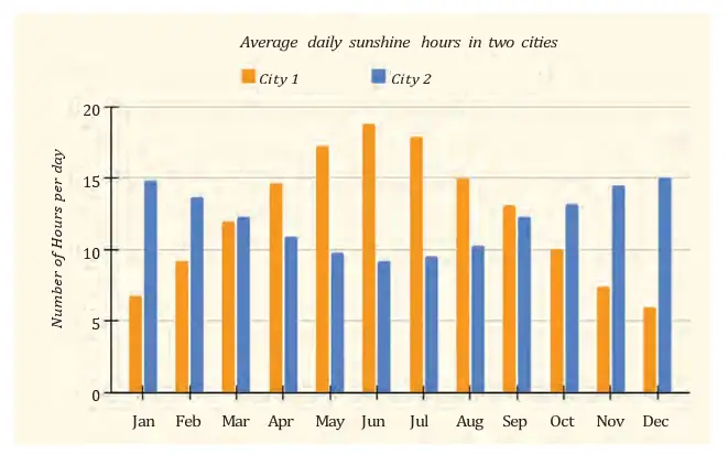
Identify, then interpret
- Identify what each axis represents and note the scale.
- Compare the bars for each month and find the highest and lowest values.
- Describe the pattern across the year, including when values rise or fall.
- Use the pattern and other relevant facts to explain what the data suggests.
What was City 1's average daily daylight in January?
- Find City 1's average daily daylight in January. January has 31 days.
- Divide its monthly total by the number of days.
- State the result with units.
Patterns and Seasonal Explanation
Main observations
- City 1: Daylight increases from January to a maximum in June, then decreases to a minimum in December. The table gives about 18.8 hours per day in June and 6 hours per day in December.
- City 2: Daylight decreases from January to a minimum in June, then increases to a maximum in December. The table gives about 9.2 hours per day in June and 15.1 hours per day in December.
- Extremes: City 1's maximum is higher and its minimum is lower than City 2's; its annual daylight variation is more pronounced.
- Day fractions: About 18 hours is three-quarters of a 24-hour day; about 6 hours is one-quarter of a day.
Why the daylight patterns are opposite
- Helsinki, Finland, is in the Northern Hemisphere; Wellington, New Zealand, is in the Southern Hemisphere.
- In June, the Northern Hemisphere tilts towards the Sun → longer days and summer in Helsinki.
- At the same time, the Southern Hemisphere tilts away from the Sun → shorter days and winter in Wellington.
- The cities are away from the Equator → their daylight hours vary more over the year.

City 2 recorded 276 daylight hours in June. Find its average daylight per day, given that June has 30 days.
Which city is likely to be in the Southern Hemisphere, and what evidence supports this?
Quick recap
- Average daily daylight = monthly daylight hours ÷ days in that month.
- Read the axes and scale before comparing bars in a clustered graph.
- City 1's daylight peaks in June and reaches its minimum in December.
- City 2's daylight reaches its minimum in June and peaks in December.
- Helsinki and Wellington have opposite daylight patterns because they are in opposite hemispheres.
- Places farther from the Equator generally have greater seasonal daylight variation.
All It Takes Is a Minute
Reading Clustered Bar Graphs
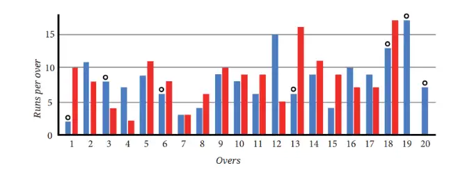
How to read a clustered bar graph
- Horizontal axis: Shows categories, such as overs, states, or times of day.
- Vertical axis: Shows the measured quantity; use the scale to read its value.
- Bars in a cluster: Each colour or pattern represents a different group or time period.
- Cricket graph: One graph unit represents 5 runs; circles indicate wickets, not runs.
Use the key and scale to read each bar. Add values across categories to compare totals; one bar alone does not show a group's total.
If a bar reaches height graph units and each unit represents data units, its value is .
Interpret a clustered bar graph
- Identify the categories, groups, units, key, and scale.
- Read the bar height and convert it to the data value using the scale.
- Add values to find totals; subtract the earlier value from the later value to find a change.
- Compare bars for the same quantity and scale; divide values to compare how many times as large.
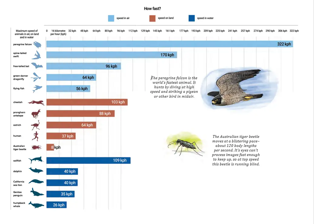
Comparing speeds
- Bar graph: Speeds can be compared with bars if the graph uses a common scale.
- About twice as fast: One speed should be close to twice the other.
- About four times as fast: Check whether the two values are close to a ratio.
- Fastest claim: A graph of selected animals cannot prove which animal is fastest in the world.
Drawing and Interpreting Graphs
Graph-drawing rules
- Scale: Choose one that fits the largest value and allows accurate plotting.
- Consistency: Use the same scale for every bar in the graph.
- Layout: Put categories on the horizontal axis and values on the vertical axis; draw matching clusters.
- Key and labels: Label the groups, axes, units, and graph.
How can the two grades' choices be shown in a double-bar graph?
- Count Grade 5 responses for aquatic (), aerial (), none (), and spaceborne ().
- Count the same choices for Grade 9.
- Use the four choices as categories and draw one bar for each grade in every cluster.
- Label both axes, add a key for the grades, and keep bar widths and spacing consistent.
| Grade | Aquatic () | Aerial () | None () | Spaceborne () |
|---|---|---|---|---|
| 5 | 6 | 12 | 4 | 2 |
| 9 | 6 | 8 | 2 | 9 |
Make a double-bar graph
- List the categories and the values for each group.
- Choose a scale that covers the largest value and mark equal intervals on the vertical axis.
- Draw equal-width bars side by side for each category, using heights set by the scale.
- Add a title, axis labels, units, and a key.
| Time | Day 1 | Day 2 |
|---|---|---|
| 12 am | ||
| 3 am | ||
| 6 am | ||
| 9 am | ||
| 12 pm | ||
| 3 pm | ||
| 6 pm | ||
| 9 pm |
Temperature comparison
- Given scale: One graph unit represents ; divide each temperature by to get its bar height.
- Likely interpretation: Day 1 is cooler and may represent a winter day; Day 2 is hotter and may represent a summer day.
- Inference: The data suggest different seasons but do not identify the exact months with certainty.
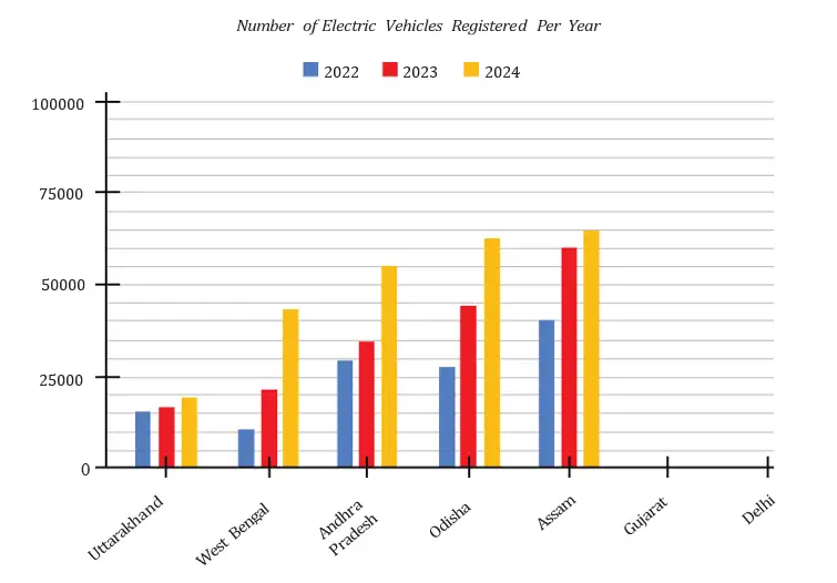
| State | 2022 | 2023 | 2024 |
|---|---|---|---|
| Gujarat | 69,000 | 89,000 | 78,000 |
| Delhi | 62,000 | 74,000 | 81,000 |
Interpreting changes
- Year clusters: Each state has one bar for each year; compare corresponding bars to see how registrations changed.
- Change: Subtract the earlier value from the later value to find an increase or decrease.
- Times as many: Divide the later value by the earlier value; a difference in bar lengths is not itself a ratio.
- Small bar difference: A small increase in bar height alone does not show that registrations were 'very few'; check the scale and values.
- Reading approximate values: Use the graph's scale and guidelines to estimate values, such as Assam's 2022–2023 change.
Use these to find the change between two years and how many times one value is another.
Do not treat bar height as the data value without applying the scale. A small-looking increase in bar length alone cannot tell you the number of registrations or the size of a percentage increase.
Using the temperature table, find the difference between the two days at 3 pm. How many graph units does each temperature represent on the given scale?
From the registration table, how much did registrations change from 2022 to 2024 in Gujarat and Delhi?
To decide which team won, compare match totals, not just a single over. For state changes, read the relevant bars using the scale before subtracting or comparing ratios.
Quick recap
- Clustered bar graphs compare two or more groups across the same categories.
- Read the key, axes, units, and scale before interpreting a bar.
- Convert bar height to data value using .
- Add values to compare totals, subtract to find changes, and divide to compare how many times as large.
- For the Grade 5 choices, the correct counts are , , , and .
- Use a consistent scale, clear labels, and a key when drawing a graph.
- A small-looking change in bar length alone does not prove that registrations were very few.
Data Detective
Reading Data Carefully
Average height — The average height for an age group is a summary of the heights of that group; it does not describe every individual.
A comparison of averages supports conclusions about the groups’ averages only; it cannot establish that every member of one group is taller than every member of another.
Average Heights in India, 1989–2019
Patterns and conclusions
- Long-term trend: The table’s average heights generally increase from 1989 to 2019 for both boys and girls at each listed age.
- Age pattern: Average height generally rises with age, but the increase from one age to the next is not always the same.
- Boys and girls: Compare values at the same age and in the same year; the taller average varies by age and year.
- Data limit: The table gives averages, not individual heights, and ends at age 19; it cannot tell us whether people keep growing after 19.
| Claim | Supported by the data? |
|---|---|
| 1. Both averages increased from 1989 to 2019 at every age. | Yes; each listed 2019 average is higher than its 1989 value. |
| 2. Girls’ average at 13 in 1989 is greater than at 14 in 2009. | No; 143.2 cm is less than 148 cm. |
| 3. Boys’ average at 15 in 2019 is greater than at 16 in 1989. | Yes; 159 cm is greater than 158.9 cm. |
| 4. Every 13-year-old girl is taller than every 11-year-old girl. | No; averages cannot establish heights of all individuals. |
| 5. Boys’ average is greater than girls’ at every age from 5 to 19. | No; for example, at age 5 in 2019 girls’ average is 107.2 cm and boys’ is 107.1 cm. |
| 6. Boys keep growing after age 19. | Cannot be concluded; the data stops at age 19. |
Comparing Growth and Making Estimates
Use this to compare average growth between two ages.
Finding the greatest increase
- Choose the year and the group (boys or girls).
- Subtract each age’s average from the next age’s average.
- Compare the differences; the largest is the greatest increase.
How much did boys’ average height increase from age 12 to 13 in 2019?
- Find the increase in boys’ average height from age 12 to 13 in 2019.
- Subtract the age-12 average from the age-13 average.
Largest increases in 2019
- Boys: The greatest increase was 6.2 cm, between ages 12 and 13.
- Girls: The greatest increase was 5.8 cm, between ages 10 and 11.
A rough 2029 estimate can extend the 1989–2019 change by one-third; it is a projection, not a measured value.
Estimating values beyond the table
- For a 2029 estimate, extend the observed 1989–2019 trend cautiously; different reasonable forecasts may vary.
- For ages 1–4, use the given newborn average of 50 cm and make a plausible increasing estimate toward the age-5 data.
- State clearly that these are estimates; the table does not provide exact values for those ages or years.
Compare the average heights of boys aged 15 in 2019 and boys aged 16 in 1989. Which is greater, and by how much?
Give one possible set of estimated average heights for young children aged 1–4, given a newborn average of 50 cm.
Using the simple decade-trend estimate, estimate boys’ average height at age 5 in 2029.
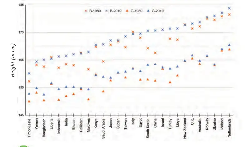
Reading a Height Visualisation
- What is shown: The visualisation compares average heights of 19-year-old boys and girls in different countries from 1989 to 2019.
- Reading the graph: Check the labels, scale and starting point of the vertical axis before comparing heights or changes.
- Interpreting values: Compare the two years for each country to describe how average heights changed over time.
Quick recap
- Compare data only after matching the group, age and year.
- The table lists average heights in India from ages 5–19 across 1989, 1999, 2009 and 2019.
- Average comparisons do not prove claims about every individual.
- Height change between successive ages is the later average minus the earlier average.
- In 2019, the largest listed increases were boys aged 12–13 and girls aged 10–11.
- Estimates beyond the available data are approximate and depend on the assumptions used.
What Do You Find Interesting?
Reading Data Displays
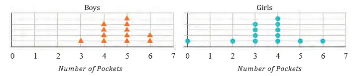
Mean and Median
| Group | Scores |
|---|---|
| 1 | |
| 2 |
Find the mean and median of Group ’s quiz scores.
- Sort the ten scores in Group .
- Add the scores and divide by ten to find the mean.
- Average the fifth and sixth values to find the median.
For an odd count, use the middle value; for an even count, average the two middle values.
Do not divide by the number of games scheduled if a player did not play all of them. Divide by games actually played; a played game with points still counts.
Player A scored ; Player B scored ; Player C scored and missed one game. Find their mean points per game and identify the best performer by this measure.
Comparing Graphs and Measurements
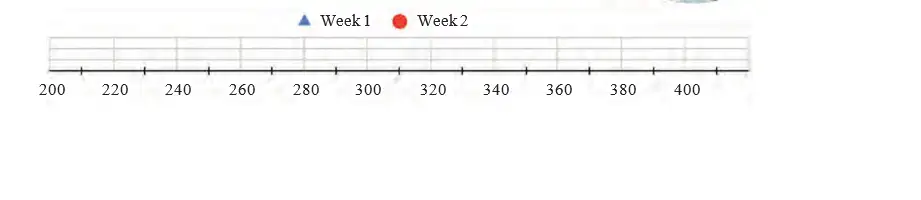
Week times are generally lower, indicating faster solving overall, though one value is comparatively high.
The heights of students are cm. Find the median and decide whether a strict height cut can make two equal-sized groups.
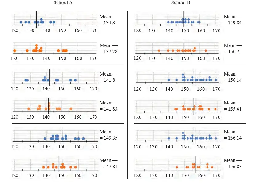
Two sections having the same numbers of boys and girls does not force their mean heights to match. Knowing one section’s mean height of cm does not determine the other section’s mean.
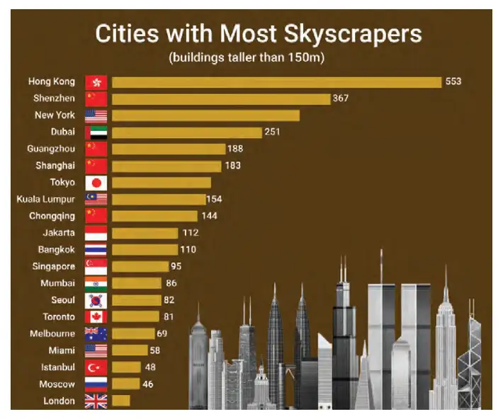
For the skyscraper graph, the first two claims about cities with more or fewer skyscrapers must be checked against the bars. A chart of skyscraper counts alone cannot show where the world’s tallest building is.
- Projects: Sentence lengths, name lengths and starting letters can be explored with dot plots, averages and frequency counts.
- Long-term data: Track daily trips out of the house for a month, then describe the centre and spread using a dot plot.
- Group investigations: Compare family heights or estimates of one- and three-minute intervals using dot plots and double-bar graphs.
Quick recap
- Check graph scales and labels before interpreting differences.
- Dot plots show individual values, frequencies, clusters and spread.
- The mean is total divided by observations; count only games actually played.
- The median is the middle value after sorting; for an even count, average the middle pair.
- Means can be affected by extreme values, so compare the median and the data distribution too.
- Use double-bar graphs for category comparisons and average absolute differences to assess estimation accuracy.
Summary
Dot Plots and Spread
Subtract the minimum value from the maximum value to find the range.
Read a Dot Plot
- Find the smallest and largest values shown.
- Count the dots at each value to identify clusters.
- Subtract the minimum from the maximum to find the range.
What do the minimum, maximum, range, and cluster tell you about this data?
- The values shown by a dot plot are .
- The minimum is , the maximum is , and is the most frequent value.
- Find the range.
Mean, Median, and Data Summaries
For ordered data, use the middle-value formula when is odd and the average of the two middle values when is even.
Find the Mean and Median
- Add all values and divide by the number of values to find the mean.
- Sort the data from least to greatest.
- Choose the middle value, or average the two middle values if the count is even.
Find the mean and median.
- Find the mean and median of the data.
- Add the values and divide by the number of values.
- The data are already sorted; the middle value is .
Do not find the median before sorting the values; for an even count, use the average of the two middle values.
Clustered Bar Graphs
Subtract the smaller value from the larger value to find how far apart two values are.
Read a Clustered Bar Graph
- Read the graph’s title, axes, scale, and legend.
- Compare the bars within a category or across categories.
- Use subtraction if you need the difference between two values.
Which group read more books in each month, and by how many?
- A clustered bar graph shows books read by two groups in two months: Month 1: Group A, ; Group B, . Month 2: Group A, ; Group B, .
- In Month 1, Group B read more; find the difference.
- In Month 2, Group A read more; find the difference.
Find the mean and median of .
A clustered bar graph shows Group A with points and Group B with points in one category. Which group has more points, and what is the difference?
Quick recap
- Dot plots make the minimum, maximum, range, and clusters visible.
- Range is the maximum value minus the minimum value.
- Mean is the sum divided by the number of values.
- Sort data to find the median; with an even count, average the two middle values.
- Minimum, maximum, total, range, mean, and median can describe and compare data.
- Clustered bar graphs compare groups across categories or time; graph patterns can prompt further questions.
Formula sheet
Mathematics — ALL CHAPTERS
1
Large Numbers Around Us
2
Arithmetic Expressions
3
A Peek Beyond the Point
4
Expressions using Letter-Numbers
5
Parallel and Intersecting Lines
6
Number Play
7
A Tale of Three Intersecting Lines
8
Working with Fractions
1
Geometric Twins
2
Operations with Integers
3
Finding Common Ground
4
Another Peek Beyond the Point
5
Connecting the Dots
6
Constructions and Tilings
7
Finding the Unknown