NEET UG . NEET Chemistry . Chemistry . Structure of Atom
Chapter 2: Structure of Atom
Ch 2
NEET Chemistry
NEET UG
Discovery of Sub-atomic Particles
Dalton’s Atomic Theory and Its Limitation
- Dalton’s theory: Proposed in 1808, it regarded the atom as the ultimate particle of matter.
- Success: It explained the laws of conservation of mass, constant composition and multiple proportions.
- Limitation: Electrical charging of substances such as glass and ebonite showed that atoms are divisible.
Discovery of the Electron
- Discovery: J. J. Thomson discovered the electron using a cathode ray discharge tube.
- Cathode rays: In a tube at low pressure and high voltage, rays travel from the cathode towards the anode.
- Conclusion: Their behaviour showed that cathode rays consist of negatively charged particles, later called electrons.
Charge-to-Mass Ratio of the Electron
Thomson’s measured value; the unit is coulomb per kilogram.
Electron Charge and Mass
Use the magnitude of the electron charge with the charge-to-mass ratio.
Protons and Canal Rays
- Discovery: E. Goldstein’s modified cathode ray tube experiment revealed positively charged particles called canal rays.
- Dependence: The charge-to-mass ratio and nature of these particles depend on the gas in the tube.
- Deflection: They bend in electric or magnetic fields in the direction opposite to cathode rays; some carry multiple units of charge.
Discovery of the Neutron
- Discovery: James Chadwick discovered neutrons by bombarding a thin sheet of beryllium with α-particles.
- Neutron: It is electrically neutral and has a mass slightly greater than that of a proton.
Properties of Fundamental Particles
How were the electron’s charge-to-mass ratio and charge determined?
State the discoveries associated with Goldstein and Chadwick.
Quick recap
- Dalton proposed in 1808 that atoms were the ultimate particles; his theory could not explain electrical charging.
- J. J. Thomson discovered electrons through cathode-ray experiments; their properties are independent of the tube’s gas and electrodes.
- Thomson measured the electron charge-to-mass ratio as .
- Millikan measured the electron’s charge; its mass is about .
- Goldstein’s canal rays were positively charged and gas-dependent; Chadwick discovered neutral neutrons.
- Protons and neutrons each have an approximate mass of , while an electron’s approximate mass is .
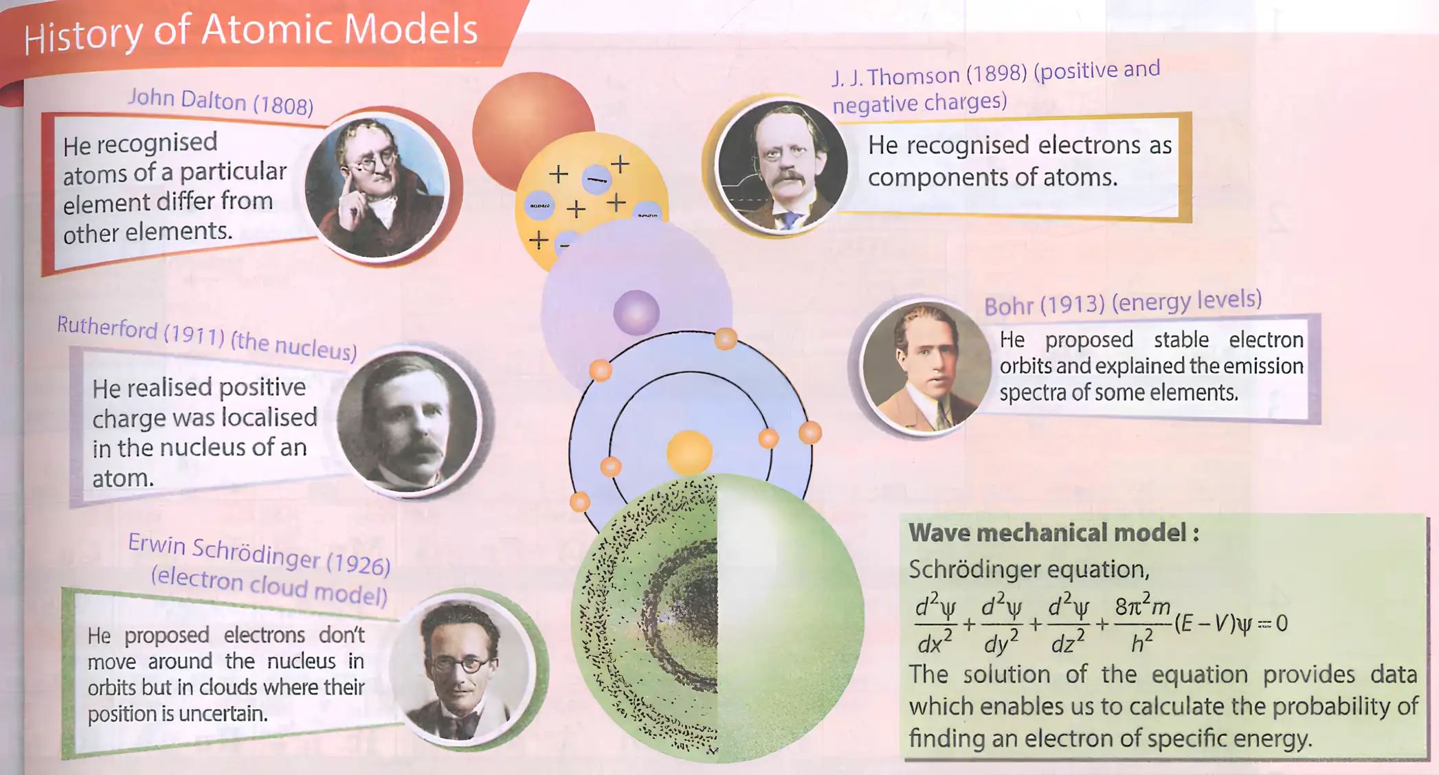
Atomic Models
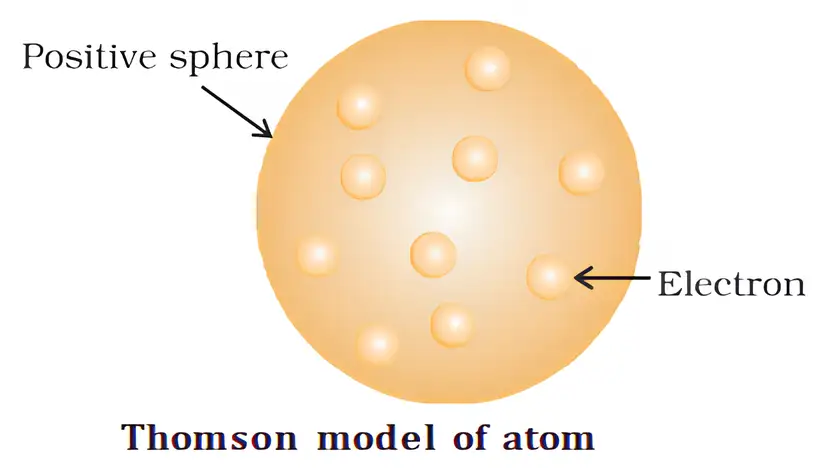
Thomson’s Model of the Atom
Thomson’s model — Proposed by J. J. Thomson in 1898: the atom is a sphere with positive charge uniformly distributed throughout it, and electrons embedded within it.
Key features and limitation
- Analogy: The positively charged sphere is like pudding, with electrons like raisins embedded in it.
- Neutrality: The electrons’ total negative charge balances the sphere’s positive charge.
- Stability: It was attributed to balance between electron–electron repulsion and attraction towards the positive sphere’s centre.
- Mass: Assumed to be distributed uniformly throughout the atom.
- Limitation: It explained overall neutrality but did not agree with results of later experiments.
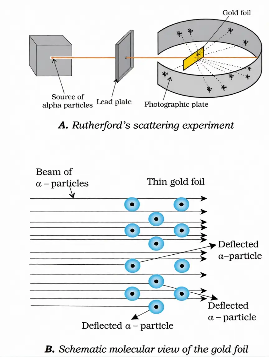
Rutherford’s Nuclear Model
Rutherford’s nuclear model — The atom has a small, dense, positively charged nucleus, with electrons moving rapidly around it in circular orbits.
Gold-foil experiment: observations and conclusions
- Most alpha-particles passed straight through: Most of an atom is empty space.
- Some alpha-particles were deflected through small or large angles: Their positive charge was repelled by a small positive centre, the nucleus, identified in 1911.
- A very few alpha-particles bounced back: The nucleus is small, dense and hard.
- Scale: Nuclear radius is about , while atomic radius is about .
- Electron motion: Electrons move at very high speed around the nucleus in circular paths called orbits.
- Solar-system analogy: The nucleus is like the Sun and orbiting electrons are like planets.
- Binding force: Electrostatic attraction holds the electrons and nucleus together.
| Order | Relative penetrating power |
|---|---|
| -rays > X-rays > -rays > -rays | -particles have the least; -particles are about 100 times and -rays about 1000 times as penetrating as -particles. |
Atomic Number, Mass Number and Related Species
Atomic number () — The number of protons in the nucleus; in a neutral atom, it also equals the number of electrons.
Mass number () — The total number of protons and neutrons (nucleons) in the nucleus.
Use these relations to determine proton, electron and neutron counts.
| Type | Defining feature | Example |
|---|---|---|
| Isotopes | Same element and atomic number; different mass numbers. | ; |
| Isobars | Different elements; same mass number but different atomic numbers. | |
| Isotones | Different elements with the same number of neutrons. | |
| Isodiaphers | Atoms with the same isotopic number, defined as number of neutrons minus number of protons. | |
| Isosters | Molecules with the same number of atoms and electrons. | |
| Isoelectronic species | Species with the same number of electrons. |
Limitations of Rutherford’s Model
Classical prediction for an orbiting electron
- An electron revolving in an orbit is accelerating because its direction of motion changes.
- Maxwell’s electromagnetic theory predicts that an accelerating charged particle emits radiation.
- The electron should lose energy and spiral towards the nucleus, causing its orbit to shrink.
- Calculations predict the electron would spiral into the nucleus in about , but atoms are stable.
What the model could not explain
- Atomic stability: It could not explain why electrons do not spiral into the nucleus.
- Electron arrangement and energy: It gave no information about how electrons are distributed around the nucleus or their energies.
What did Rutherford infer from the gold-foil experiment?
Why could Rutherford’s model not account for atomic stability?
Quick recap
- Thomson’s 1898 model pictured electrons embedded in a sphere with positive charge uniformly distributed throughout it.
- Rutherford’s gold-foil experiment showed that most of the atom is empty space and pointed to a small, dense, positive nucleus.
- Some alpha particles were deflected through small angles and others through larger angles; very few were thrown back.
- Nuclear radius is about ; atomic radius is about .
- Atomic number is the proton count; mass number is the sum of proton and neutron counts.
- Distinguish isotopes, isobars, isotones, isodiaphers, isosters and isoelectronic species by their defining counts.
- Rutherford’s model could not explain atomic stability or the distribution and energies of electrons.
Developments Leading to the Bohr’s Model of Atom
Wave Nature of Electromagnetic Radiation
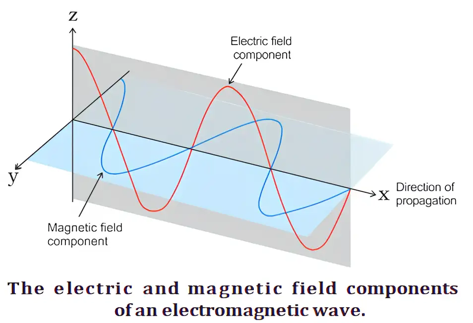
In vacuum, electromagnetic waves travel at the speed of light; frequency and wavelength are inversely related.
Wavenumber is the reciprocal of wavelength.
Frequency and wavelength
- Higher frequency: Corresponds to a shorter wavelength.
- Lower frequency: Corresponds to a longer wavelength.
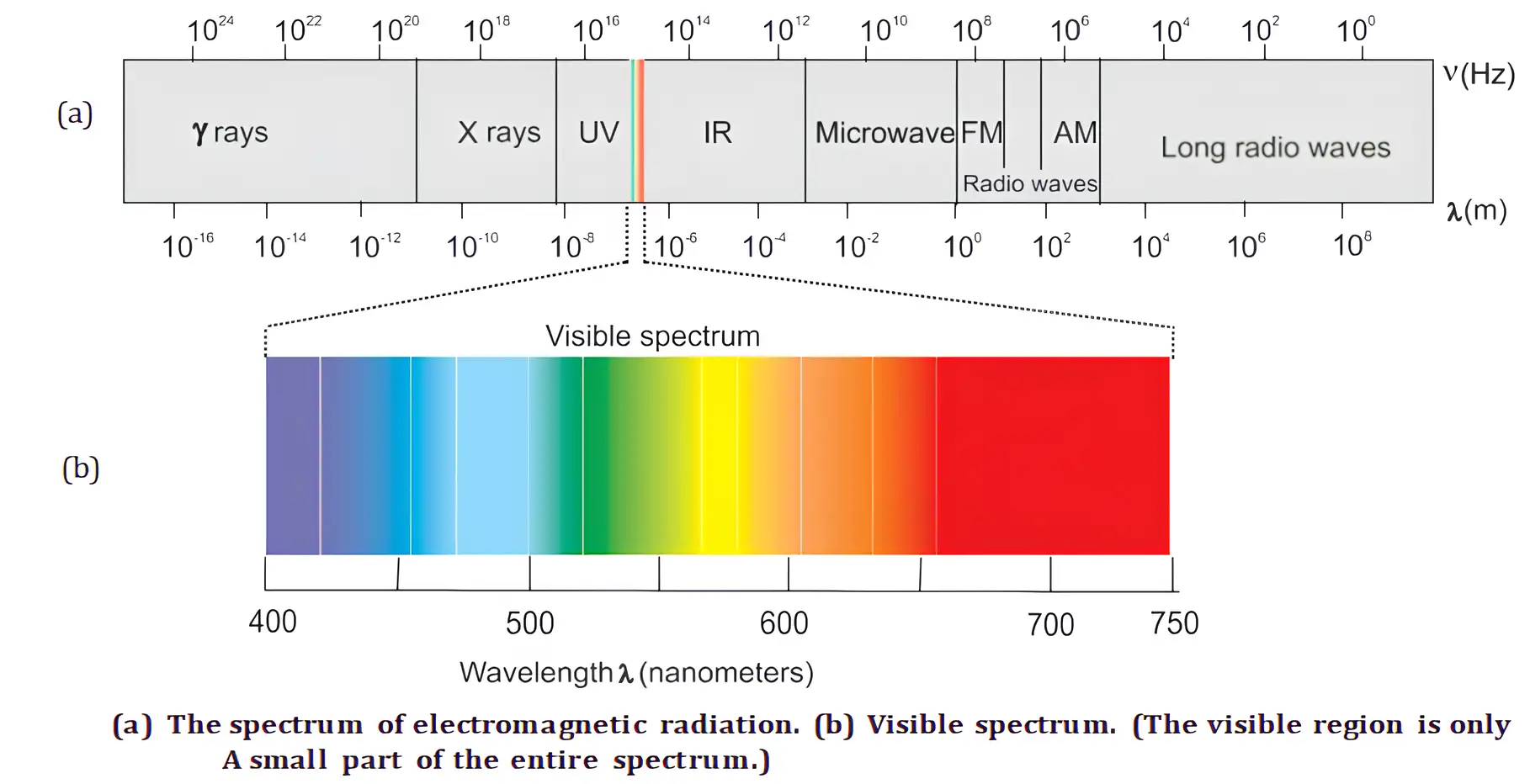
Electromagnetic spectrum — The arrangement of electromagnetic radiations in order of increasing wavelength or decreasing frequency.
Black-Body Radiation and Planck’s Quantum Theory
Black body — An ideal body that emits and absorbs radiation of all frequencies.
Black-body radiation — The radiation emitted by a black body.
Planck’s quantum theory
- Quantized exchange: Atoms and molecules emit or absorb energy only in discrete packets, not continuously.
- Quantum: The smallest quantity of energy emitted or absorbed as electromagnetic radiation.
- Planck’s constant: .
The energy of a quantum is proportional to the radiation frequency.
The total energy is an integer multiple of one quantum; is an integer.
Photoelectric Effect
Photoelectric effect — The ejection of electrons from certain metals, such as K, Rb and Cs, when exposed to light at or above a minimum frequency.
Threshold frequency and work function
- Threshold frequency (): The minimum frequency needed to eject electrons from the metal.
- Work function (): The minimum energy required to eject an electron.
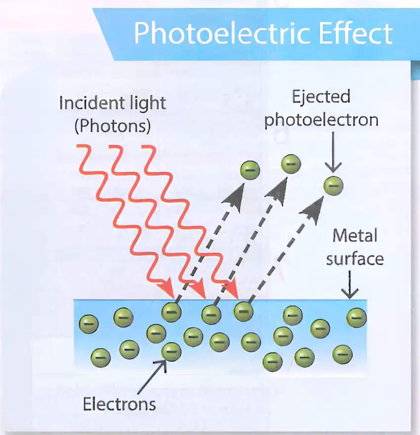
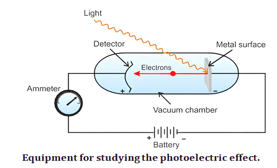
Incident photon energy supplies the work function and the ejected electron’s kinetic energy.
Dual Nature of Electromagnetic Radiation
Dual nature of light — Light behaves as a wave while propagating and as a stream of particles when interacting with matter.
Spectra and Hydrogen Spectral Series
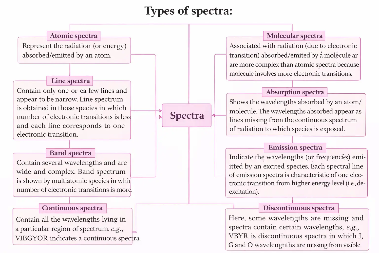
Spectrum — The combination of lights of different wavelengths analysed through a prism.
| Series | Final level () | Possible upper levels () | Spectral region |
|---|---|---|---|
| Lyman | Ultraviolet | ||
| Balmer | Visible | ||
| Paschen | Infrared | ||
| Brackett | Infrared | ||
| Pfund | Infrared |
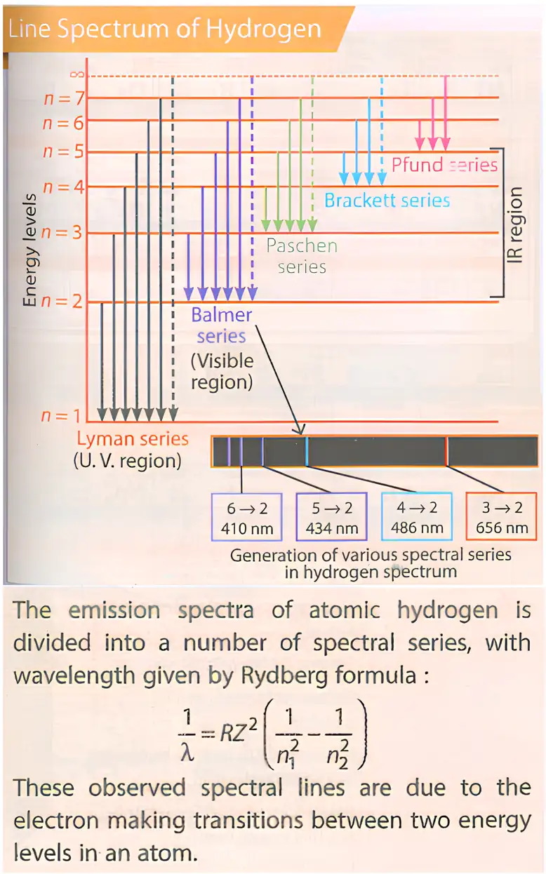
For an electron initially at level , the maximum number of lines produced as it returns to level is given by this expression.
For an electron returning from level to level , the number of possible spectral lines is:
State Planck’s quantum relation and the total-energy expression.
Define the photoelectric effect and write its energy equation.
Name the hydrogen spectral series and give their spectral regions.
Quick recap
- Maxwell’s wave theory describes energy as emitted continuously and travelling as electromagnetic waves.
- Electromagnetic waves have mutually perpendicular electric and magnetic fields; in vacuum, .
- Frequency and wavelength vary inversely, and wavenumber is .
- A black body emits and absorbs all frequencies; Planck’s theory describes energy in discrete packets: and .
- Photoelectric ejection requires at least the threshold frequency; is the work function.
- Light behaves as a wave during propagation and as particles during interaction with matter.
- Hydrogen spectral series are classified by final level; their line counts follow the stated formulas.
Bohr’s Model for Hydrogen Atom
Orbits and Energy Transitions
Bohr orbit — A Bohr orbit is a permitted path around the nucleus with a fixed radius and fixed energy.
Energy changes
- Stationary orbit: An electron’s energy remains constant while it stays in a permitted orbit.
- Absorption: Moving from a lower to a higher energy level requires energy absorption.
- Emission: Moving from a higher to a lower level releases energy as radiation.
- Level order: ; successive energy gaps decrease as the level rises.
For a transition from level 1 to level 2, the absorbed or emitted energy equals the level difference.
Quantisation of Angular Momentum
- Allowed orbits: An electron can occupy only orbits whose angular momentum is an integral multiple of .
- Quantum number: identifies the orbit; is the electron mass and its orbital speed.
Energy of Hydrogen-like Species
- Hydrogen-like species: A one-electron atom or ion; examples include hydrogen, , and .
- Nuclear charge: is the atomic number; for a hydrogen-like species, the energy depends on and .
- Rydberg energy constant: .
The negative sign indicates a bound electron; the zero-energy reference is an electron infinitely far from the nucleus.
Use the form appropriate to the energy units required.
Radius of Bohr Orbits
| Species | Radius of the nth orbit | Dependence |
|---|---|---|
| Hydrogen atom | ||
| Any hydrogen-like species with nuclear charge |
- Bohr radius: for the first orbit of hydrogen.
This form gives the radius of the nth orbit for a hydrogen-like species.
Ionisation Energy and Electron Velocity
Ionisation takes the electron from level to infinity, where its energy is zero.
For a hydrogen-like species, velocity increases with nuclear charge and decreases with principal quantum number.
This is the constant form of the velocity of an electron in the nth shell of a hydrogen-like species.
Rydberg Formula
- Use: Relates the wavelength of radiation to a transition between two energy levels in hydrogen or a hydrogen-like species.
- Levels: ; the formula gives the spectral-line wavenumber, .
; is the atomic number.
Limitations of Bohr’s Theory
- Multi-electron atoms: Could not explain the spectra of atoms containing more than one electron.
- Electron distribution: Did not satisfactorily explain how electrons are distributed within an atom.
- External fields: Could not explain spectral-line splitting in a magnetic field (Zeeman effect) or electric field (Stark effect).
- Modern principles: Ignored the wave–particle duality of matter and the uncertainty principle.
State Bohr’s angular-momentum condition.
Give two limitations of Bohr’s theory.
Quick recap
- Electrons occupy permitted orbits with fixed radii and energies.
- Transitions between levels absorb or emit energy equal to .
- Allowed angular momenta are integral multiples of .
- For hydrogen-like species, and .
- Ionisation energy is the energy needed to move an electron from its orbit to infinity.
- The Rydberg formula relates spectral-line wavelength to transitions between energy levels.
- Bohr’s model fails for multi-electron spectra, field-induced line splitting and modern quantum principles.
Towards Quantum Mechanical Model of the Atom
Wave–Particle Duality and de Broglie’s Equation
Wave–particle duality — An electron has both particle-like and wave-like properties.
de Broglie waves
- de Broglie’s proposal: Every moving object has an associated wave; the waves are not radiated away into space.
- Wavelength: It is inversely proportional to momentum, so greater mass at a given speed gives a shorter wavelength.
- Significance: The wavelength is measurable for subatomic particles such as electrons, but is negligible for ordinary large objects.
Here, is Planck’s constant and is the particle’s momentum.
For a particle of mass , charge , and accelerating potential , its kinetic energy is .
Heisenberg’s Uncertainty Principle
Heisenberg’s uncertainty principle — It is impossible to determine simultaneously the exact position and exact momentum of an electron.
Here, is position uncertainty and is momentum uncertainty; for a particle of mass , .
Significance
- Electron paths: The principle rules out definite paths or trajectories for electrons and similar microscopic particles.
- Scale: It is significant for microscopic particles but negligible for macroscopic objects.
State de Broglie’s equation and explain what it shows.
What does Heisenberg’s uncertainty principle imply about an electron’s path?
Quick recap
- Moving particles have wave character; an electron’s associated wave is not radiated away.
- The de Broglie wavelength is and decreases as momentum increases.
- For a particle accelerated through potential , .
- Position and momentum uncertainties obey .
- The uncertainty principle rules out definite electron trajectories and matters chiefly for microscopic particles.
Quantum Mechanical Model of Atom
Quantum Mechanical Model
Wave function and orbitals
- Schrödinger wave equation: A mathematical equation whose allowed solutions describe the wave-like behaviour of an electron in an atom.
- Wave function (): It has no direct physical significance; gives the probability density of finding an electron at a point.
- Atomic orbital: A three-dimensional region around the nucleus where the probability of finding an electron is maximum.
- Probability density: is always non-negative; the probability of finding an electron in a small volume depends on the value of there.
Key Features of the Quantum Mechanical Model
- Quantized energy: Electrons in atoms can have only certain allowed energy values; these arise from allowed wave solutions of the Schrödinger equation.
- Uncertainty principle: The exact position and exact velocity of an electron cannot both be known simultaneously.
- Orbital wave function: An atomic orbital is the wave function for an electron in an atom.
- Probability: The probability density at a point is proportional to at that point.
Quantum Numbers
Quantum numbers — Four numbers that together specify the state of an electron in an atom.
| Quantum number | Allowed values | What it tells us |
|---|---|---|
| Principal, | Positive integers: ; shells correspond to | Main shell, approximate distance and energy; shell capacity is . Explains the main lines of the spectrum. Bohr angular momentum: . |
| Azimuthal, | For a given : to ; , , , | Subshell, orbital shape and relative subshell energies; fine structure of spectral lines. Orbital angular momentum: . |
| Magnetic, | For a given : integer values from to , including | Orbital orientation in space, number of orbitals in a subshell and splitting of spectral lines in a magnetic field. |
| Spin, | or | Electron spin direction and magnetic properties. Spin angular momentum: , where . |
For a shell with principal quantum number , and a subshell with azimuthal quantum number . The maximum electrons are twice the number of orbitals.
Using the quantum numbers
- Orbitals in a subshell: The values of run from through , giving orbitals.
- Electrons per orbital: Each orbital can hold at most two electrons, with opposite spins.
Shapes of Atomic Orbitals and Nodes
- Born interpretation: Max Born interpreted at a point as the electron probability density there.
- Orbital shape: It is determined by the total probability density, including both radial and angular contributions.
- Nodes: A node is a region or surface where the probability density is zero.
For an orbital with quantum numbers and .
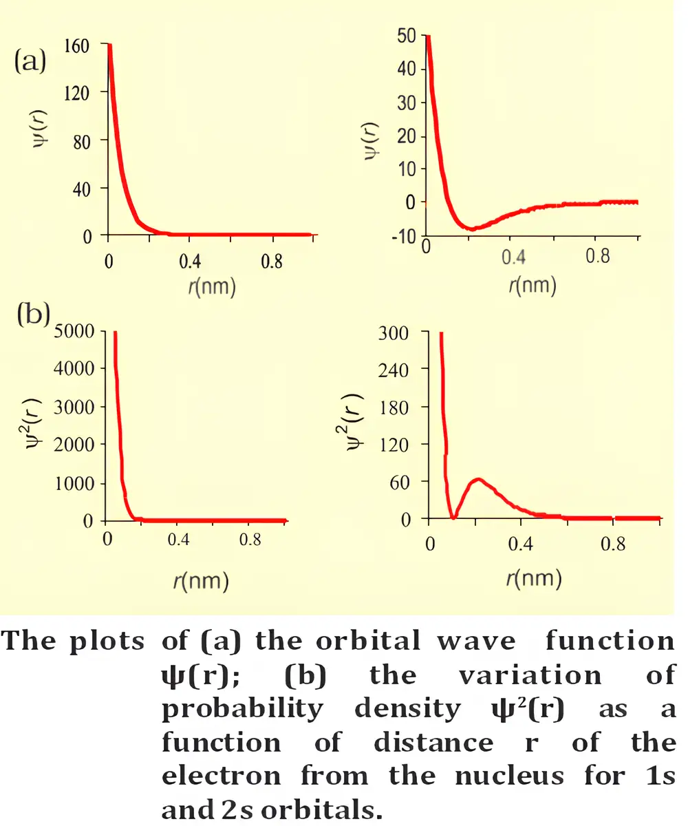
Probability density and orbital shapes
- orbital: Probability density is greatest at the nucleus and falls as distance increases.
- orbital: Its probability density reaches zero at a radial node, rises to a smaller maximum, then decreases towards zero as increases.
- orbitals: Spherical, because the probability of finding the electron is equal in every direction at a given distance from the nucleus.
- orbitals: Dumb-bell shaped, with two lobes on opposite sides of the nucleus; , and point along the respective axes. Each has one nodal plane through the nucleus.
- orbitals: There are five: , , , and . Most are cloverleaf-shaped; has a distinctive doughnut-shaped region.
- nodes: Each orbital has two nodal planes.
Energy of Orbitals
- Hydrogen atom: Orbital energy depends only on ; orbitals with the same are degenerate (equal in energy). Thus, and have equal energy in hydrogen.
- Ground state: The orbital is the most stable state in hydrogen; an electron in , or a higher orbital is in an excited state.
- Multi-electron atoms: Orbital energy depends on both and , unlike in hydrogen.
- rule: Lower means lower energy; if two orbitals have the same , the orbital with lower has lower energy.
- Effective nuclear charge: Within the same subshell, orbital energy decreases as effective nuclear charge increases.
- Common energy order: .
The energy rule
Lower fills first; in a tie, lower fills first.
Filling of Orbitals
| Rule | Statement |
|---|---|
| Aufbau principle | In the ground state, electrons occupy orbitals in order of increasing energy. |
| Pauli exclusion principle | No two electrons in an atom have the same set of four quantum numbers; one orbital holds at most two electrons, with opposite spins. |
| Hund’s rule of maximum multiplicity | Within a subshell, electrons occupy each orbital singly before any pairing occurs. |
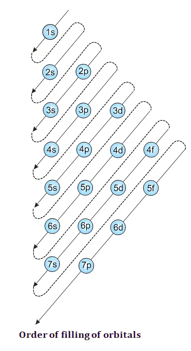
Aufbau filling order
- Order:
Electronic Configuration and Stability
Electronic configuration — The distribution of an atom’s electrons among its orbitals according to the orbital-filling rules.
Why half-filled and fully filled subshells can be especially stable
- Symmetry: Half-filled and completely filled subshells have more symmetrical electron distributions, which contributes to stability.
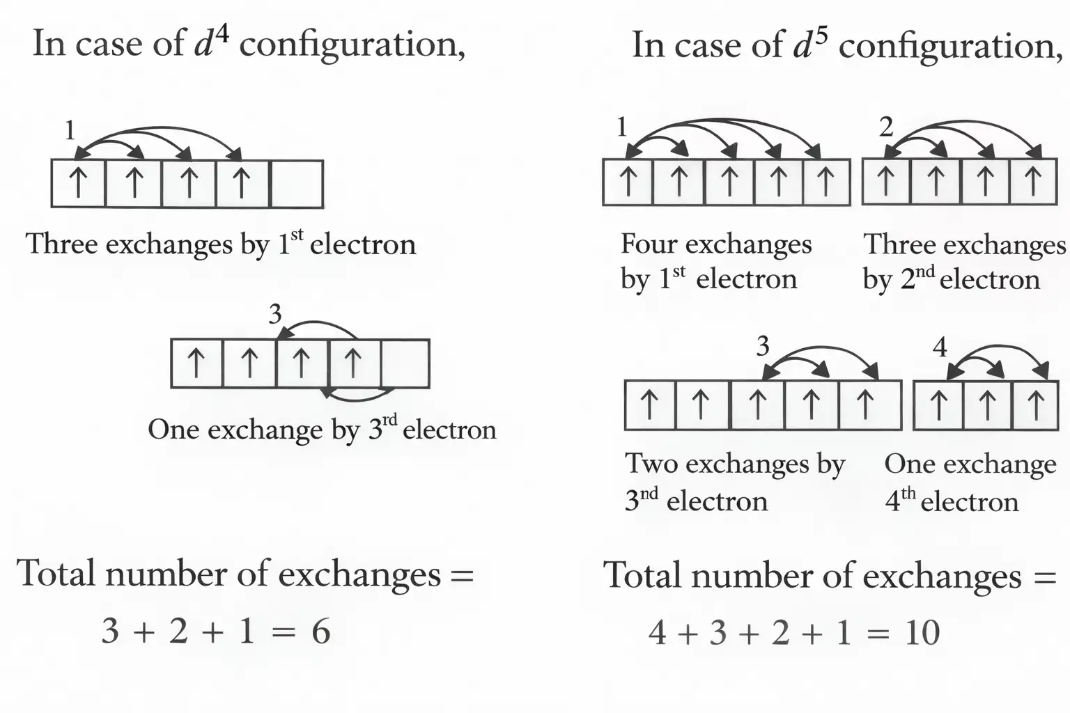
- Exchange energy: Electrons in different orbitals of the same subshell can exchange positions; each possible exchange releases energy.
- Maximum exchange: Exchange opportunities are greatest for exactly half-filled and fully filled arrangements, so these arrangements gain extra stability.
- Examples: A arrangement has more exchange possibilities than ; has more than .
State the three rules used to fill orbitals.
How many radial, angular and total nodes does an orbital have?
Quick recap
- The wave function describes an orbital; gives probability density.
- Four quantum numbers specify an electron’s shell, subshell, orbital orientation and spin.
- Shell capacity is ; a subshell has orbitals and can hold electrons.
- Node counts are radial , angular , and total .
- For multi-electron atoms, use the rule and then lower to compare orbital energies.
- Orbital filling follows Aufbau, Pauli exclusion and Hund’s rule.
- Half-filled and fully filled subshells can gain extra stability through symmetry and exchange energy.
NEET Chemistry — ALL CHAPTERS
1
Some Basic Concepts of Chemistry
2
Structure of Atom
3
Classification of Elements and Periodicity in Properties
4
Chemical Bonding and Molecular Structure
5
Thermodynamics
6
Equilibrium
7
Redox Reactions
8
Organic Chemistry - Some Basic Principles and Techniques
9
Hydrocarbons
10
Solutions
11
Electrochemistry
12
Chemical Kinetics
13
The d- and f- Block Elements
14
Coordination Compounds
15
Haloalkanes and Haloarenes
16
Alcohols, Phenols and Ethers
17
Aldehydes, Ketones and Carboxylic Acids
18
Amines
19
Biomolecules
20
The p-Block Elements (Group 13 and 14)
21
The p-Block Elements (Group 15 to 18)
22
Principles Related to Practical Chemistry