NEET UG . NEET Physics . Physics . Basic Mathematics
Chapter 1: Basic Mathematics
Ch 1
NEET Physics
NEET UG
Slope
Meaning and Calculation of Slope
- Definition: Slope measures the steepness of a line and is the ratio of vertical change to horizontal change.
- Formula: For points and , , where is the angle with the positive x-axis.
- Line equation: In , is the slope and is the y-intercept.
- Types: Positive slope rises, negative slope falls, zero slope is horizontal, and an undefined slope is vertical.
- Relations: Parallel lines have equal slopes; perpendicular lines have .
Quick recap
- Slope is rise divided by run: .
- For two points, .
- In , is the slope and is the -intercept.
- Positive, negative, zero and undefined slopes correspond to rising, falling, horizontal and vertical lines.
- Parallel lines have equal slopes; perpendicular lines satisfy .
- The angle formula is .
Area
Graphical Representation of Area
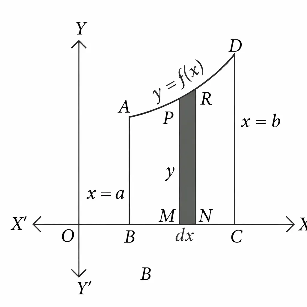
- Region: The area under from to is represented using vertical strips.
- Strip area: A thin strip at position has height , width , and area approximately .
- Integral: Adding the strips gives when the curve lies above the x-axis.
Quick recap
- A continuous curve on can be divided into thin vertical strips.
- Each strip has height and width .
- A strip’s area is .
- Adding the strips gives for a curve above the -axis.
Straight Line Graph
Meaning of a Linear Graph
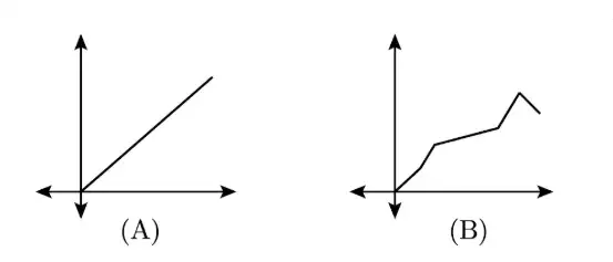
Linear graph — A linear graph represents a linear equation in two variables as a straight line and shows a linear association between two quantities.
General Form
- Equation: , where , and are real numbers, with and .
- Graph: The solution pairs of the equation lie on its straight-line graph.
Using a Graph to Model Earnings
Hourly Pay and Daily Savings
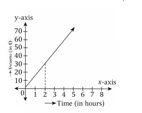
- Model: James earns 15 dollars per hour. If he works for hours, his income is given by .
- Savings condition: With a daily expenditure of 50 dollars, he saves money when , or hours.
- Graph reading: Income is read on the vertical axis; the corresponding time on the horizontal axis shows how long he must work to earn more than 50 dollars.
- Example: At 5 hours, income is 75 dollars and savings are dollars.
| Point | Linear graph | Line graph |
|---|---|---|
| Shape | A straight-line graph representing a linear relationship. | Can consist of connected segments that do not form one straight line. |
| In the figure | Graph A is a straight line. | Graph B is piecewise and irregular. |
Important Graphing Points
Plotting and Special Straight Lines
- Plotting points: Two solution pairs are sufficient to draw a straight line, but an incorrect pair may go unnoticed.
- Check: Plot a third point to verify that the equation’s solutions have been obtained correctly.
- Horizontal line: , where is real, is parallel to the -axis.
- Vertical line: , where is real, is parallel to the -axis.
A line parallel to the -axis.
A line parallel to the -axis.
Quick recap
- Linear graph: The graph of a linear equation in two variables is a straight line.
- General form: , where , and are real, and and are nonzero.
- Earnings model: James's income after hours is ; he saves when hours.
- Example: At 5 hours, income is 75 dollars and savings are 25 dollars.
- Plotting: Two points draw a straight line; a third point helps check the plotted solutions.
- Special lines: is horizontal and is vertical.
Inverse Function
Meaning and existence of an inverse
Inverse function — The inverse of a function is written and reverses the mapping made by .
- Domain and range: The domain of becomes the range of ; the range of becomes the domain of .
- Existence: is a function only when is both one-one and onto (bijective).
- Composition: Applying a function and its inverse in either order returns the input: .
Do not confuse with . The inverse function undoes ; the reciprocal is a different function.
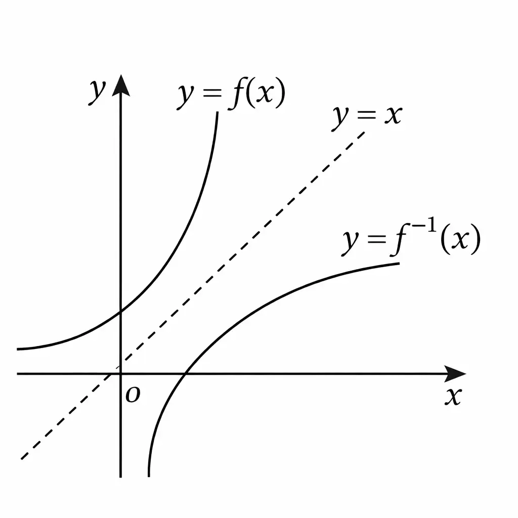
Graph of an inverse function
- Coordinate swap: If lies on , then lies on .
- Reflection: The graphs of inverse functions are reflections of one another across .
- Inverse pair test: If , then and .
Common inverse mappings
- Families: Common inverse functions include inverse trigonometric, rational, hyperbolic and logarithmic functions.
| Function | Inverse | Conditions or range |
|---|---|---|
| Inverse operation: subtract the added constant. | ||
| and | ||
| Restrict the original domain to ; then . | ||
| ; choose a suitable domain for a one-one function. | ||
| , , and | ||
| Restrict the original domain to ; inverse range is . | ||
| Restrict the original domain to ; inverse range is . | ||
| Restrict the original domain to ; inverse range is . |
State the condition for a function to have an inverse function.
How are the graphs of a function and its inverse related?
Quick recap
- An inverse function reverses the mapping of the original function.
- The inverse exists as a function when the original function is bijective.
- The domain and range swap between a function and its inverse.
- Inverse graphs are reflections across .
- Composing a function with its inverse in either order gives the identity mapping.
- Common inverses include roots, logarithms and inverse trigonometric functions.
Parabola
Parabola: definition and forms
- Definition: A parabola is the locus of points equidistant from a fixed point, called the focus, and a fixed line, called the directrix.
- Forms: A parabola can be written as or , with vertex .
Standard parabola and its parts
For , the directrix is (not ); the latus rectum length is positive, for .
Graph and features from a quadratic
- Opening: For , the sign of determines the direction: it opens upward if and downward if .
- Vertex and symmetry: The vertex has x-coordinate , and the axis of symmetry is the vertical line through the vertex.
- Example: For , the vertex is , the axis is , and the parabola opens upward.
Basic differentiation formulas
Chain rule — For a composite function with and , differentiate the outer function with respect to , then multiply by the derivative of with respect to .
Use for a composite function.
Differentiation as a rate of change
The derivative is the limiting average rate of change.
Rate of change of two variables and slope
This gives the slope or rate of change of with respect to .
Quick recap
- A parabola is equidistant from its focus and directrix; its eccentricity is .
- Vertex forms give the vertex, axis, opening direction, focus, and directrix.
- For , the focus is , directrix , and latus rectum length .
- For , the vertex has and .
- Differentiation gives instantaneous rate of change; the chain rule handles composite functions.
- For parametric variables, when .
Application of Derivative
Slope of a Secant
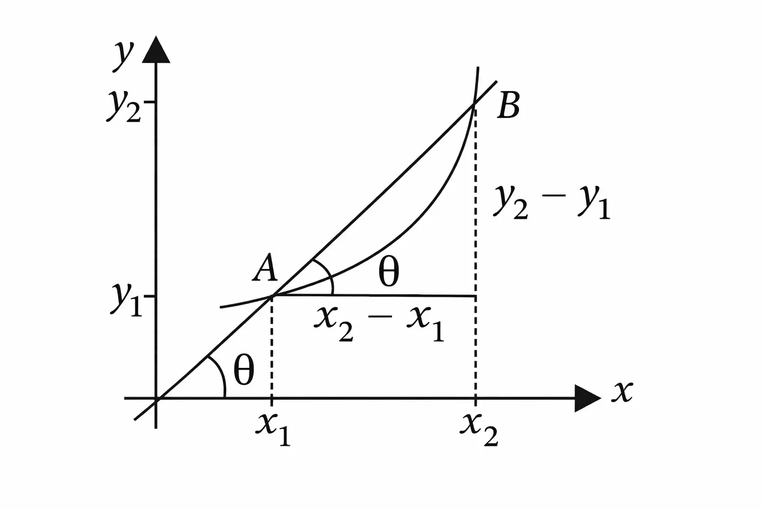
Secant slope — The slope of the line joining two points on a curve is the change in divided by the change in .
Key idea
- Secant: A straight line through two points on a curve.
- Slope: For points and , slope is .
Slope of a Tangent
Tangent — A tangent is the limiting position of a secant when its two points approach the same point on the curve.
Derivative as slope
- Limit: As , the secant approaches the tangent at the point.
- Derivative: The derivative gives the slope of the tangent to the curve at that point.
- Angle: If the tangent makes angle with the -axis, its slope is .
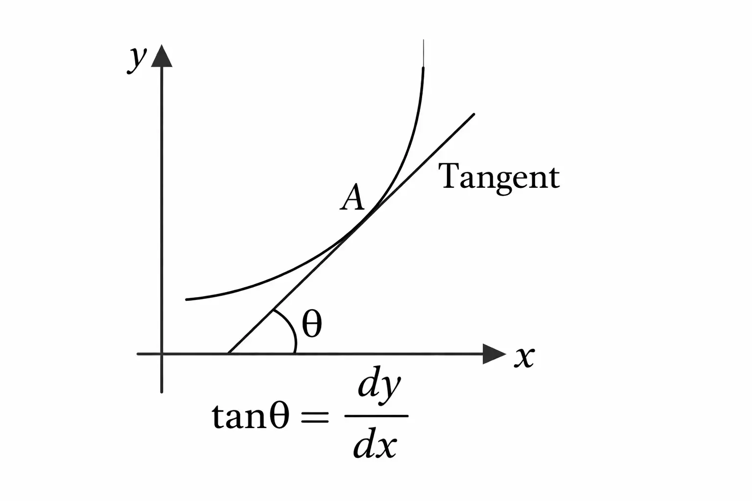
Maxima and Minima
Stationary points
- Maximum: At a maximum, the tangent is horizontal, so its slope and first derivative are zero.
- Minimum: At a minimum, the tangent is also horizontal, so its slope and first derivative are zero.
- Stationary condition: Maxima and minima occur at points where .
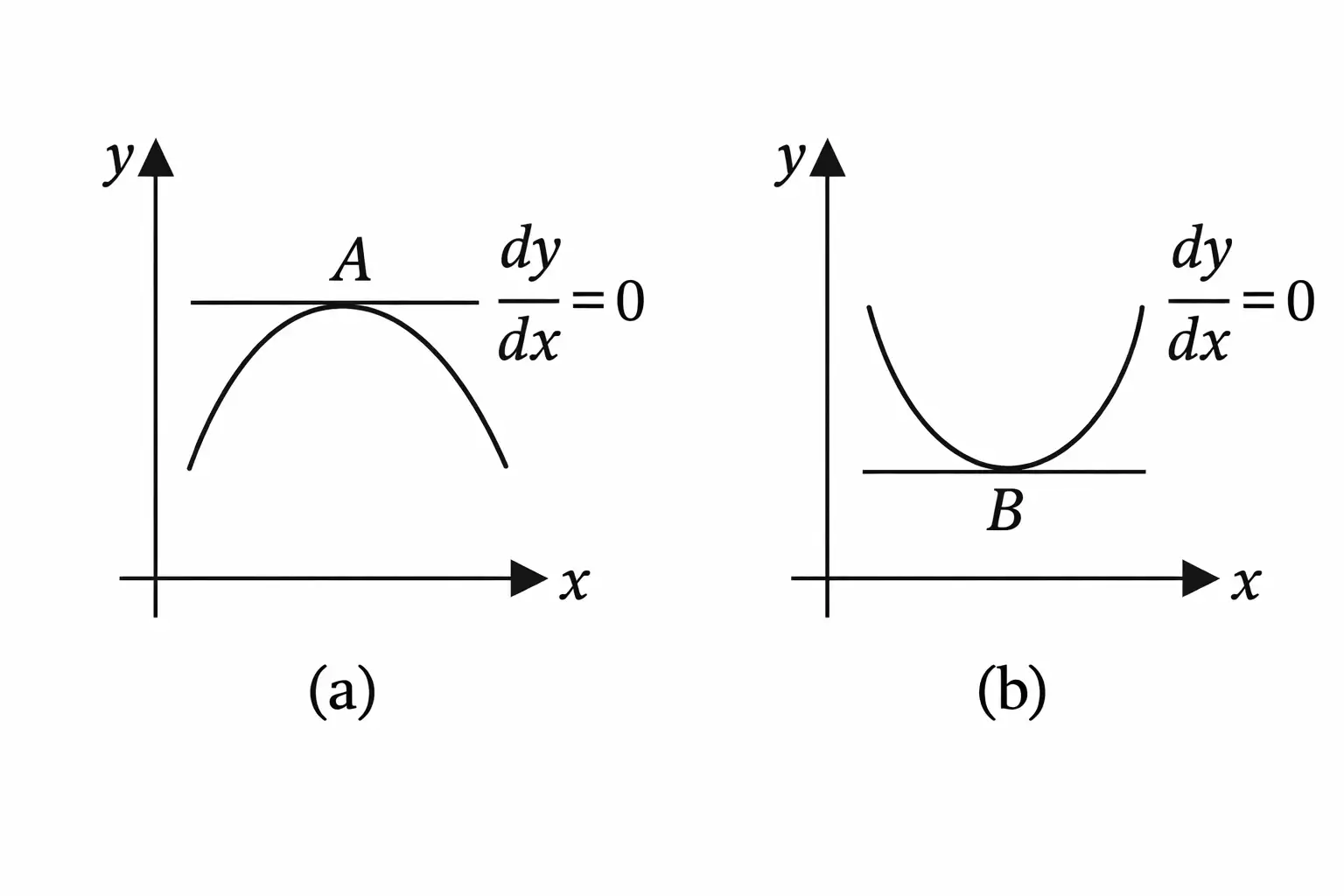
| At a stationary point | Nature of point |
|---|---|
| Maximum | |
| Minimum |
How is the slope of a tangent related to the derivative?
How does the second derivative distinguish a maximum from a minimum?
Quick recap
- Secant slope is .
- A tangent is the limiting position of a secant as its two points coincide.
- The derivative is the tangent slope and equals .
- At a maximum or minimum, the tangent is horizontal and .
- At a stationary point, a negative second derivative indicates a maximum.
- At a stationary point, a positive second derivative indicates a minimum.
Integration
Standard Integration Formulae
| Function | Integral |
|---|---|
Indefinite Integration
Indefinite integral — Integration reverses differentiation: an indefinite integral gives a family of antiderivatives, differing by a constant.
Use for powers other than ; is the arbitrary integration constant.
- Check: Differentiating the result of an indefinite integral must recover the original integrand.
- Exception: For , use rather than the power rule.
Integration by Substitution
Substitution — A change of variable that converts an integral into a standard form that is easier to evaluate.
If the integrand contains a function and the derivative of its inner expression, set that inner expression equal to a new variable.
| Integrand pattern | Substitution |
|---|---|
Choosing a substitution
- Look for: An inner function whose derivative also appears in the integrand, possibly multiplied by a constant.
- Then: Replace the inner function with a new variable, rewrite the differential, integrate, and substitute back.
- Choice: There is no single rule for every integral; choose the substitution that simplifies the integrand.
Definite Integration
Definite integral — An integral evaluated between a lower limit and an upper limit; its value is obtained from an antiderivative at those limits.
If , evaluate the antiderivative at the upper limit, then subtract its value at the lower limit.
Rules for Integration
A constant factor can be taken outside the integral.
Integrate each function separately; retain the plus or minus sign.
How is a definite integral evaluated?
When is substitution useful?
Quick recap
- Integration reverses differentiation; an indefinite integral includes an arbitrary constant .
- Use the power rule for ; integrate as .
- Standard integrals include the basic trigonometric functions and .
- Substitution replaces a suitable inner function with a new variable and changes the differential accordingly.
- For a definite integral, evaluate the antiderivative at the upper limit minus its value at the lower limit.
- Constants factor out of integrals, and sums or differences can be integrated term by term.
Area Under Simple Curves
Area Under a Curve
The integral adds the areas of the strips between and .
Quick recap
- A continuous curve on can be divided into thin vertical strips.
- Each strip has height and width .
- The definite integral adds the areas of the strips from to .
- The area is expressed as .
Circumferences of Circle
Arc Length and Circumference
Circumference — The circumference is the total length around a circle.
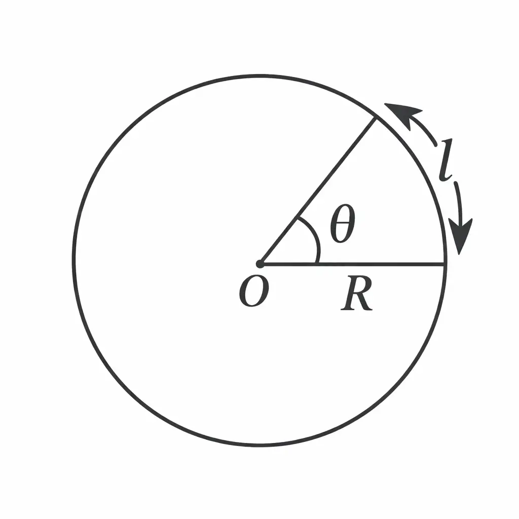
Arc Length and Circumference
- Arc element: For a small angle measured in radians, the arc length is .
- Full circle: Integrate over angles from to to obtain the circumference.
For a circle of radius .
Area of a Circle
Area of a circle — The area of a circle is the region enclosed by its circumference.
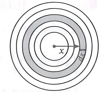
Annular-Strip Derivation
- Strip area: At distance from the centre, a thin ring of thickness has area .
- Whole circle: Add the ring areas from to .
For a circle of radius .
Volume of a Sphere
Volume of a sphere — The volume of a sphere is the space enclosed by its surface.
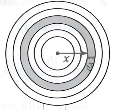
Thin-Shell Derivation
- Shell volume: A thin spherical shell at radius has surface area , so its volume is .
- Whole sphere: Integrate the shell volumes from the centre, , to the outer radius, .
For a sphere of radius .
Cylinder and Triangle Formulas
| Shape or measure | Formula |
|---|---|
| Right circular cylinder, area as stated in the source | |
| Right circular cylinder, volume | |
| Triangle with base and altitude , area |
How is the circumference of a circle obtained from the arc-length element?
State the formulas for the area of a circle and the volume of a sphere.
Quick recap
- For a small angle in radians, the arc-length element is .
- A circle of radius has circumference and area .
- A thin annular strip at radius has area .
- A thin spherical shell at radius has volume .
- A sphere of radius has volume .
- A cylinder has volume and the stated area formula is .
- A triangle with base and altitude has area .
Simultaneous Equation
Pairs of Linear Equations
Pair of linear equations in two variables — Two linear equations involving the same two variables form a pair, or system, of simultaneous linear equations.
The coefficients are real, and each equation must contain at least one non-zero coefficient of its variables.
Example
- Example: and form a pair of linear equations in and .
Solutions and Graphical Representation
Solution of a pair — An ordered pair that satisfies both equations simultaneously is a solution of the pair.
Graphical meaning
- Line: Each linear equation in two variables represents a straight line; a pair of equations represents two lines.
- Plotting: At least two points (solutions) are needed to draw each line.
- Intersection: The intersection coordinates satisfy both equations and give the unique solution.
- Parallel lines: They do not meet, so the pair has no solution.
- Coincident lines: They overlap; every point on the line is a solution, giving infinitely many solutions.
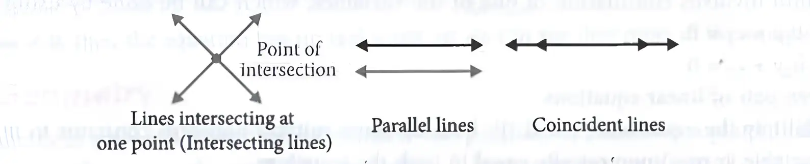
Consistency Conditions and Unknown Constants
| Coefficient ratios | Graph | Solutions | Consistency |
|---|---|---|---|
| Intersecting lines | Exactly one solution | Consistent | |
| Parallel lines | No solution | Inconsistent | |
| Coincident lines | Infinitely many solutions | Consistent and dependent |
Algebraic Methods for Two Variables
Substitution method
- 1. Express: Rearrange one equation to write one variable in terms of the other, such as in terms of .
- 2. Substitute: Insert that expression into the other equation and solve the resulting one-variable equation.
- 3. Recover: Substitute the found value into the rearranged equation to find the second variable.
- Check: A true statement with no variable means infinitely many solutions; a false statement means no solution.
Elimination method
- 1. Match coefficients: Multiply the equations by suitable non-zero constants so one variable has equal or opposite coefficients.
- 2. Eliminate: Add or subtract the equations to remove that variable.
- 3. Solve and substitute: Solve the resulting one-variable equation, then substitute to find the other variable.
- Check: A true variable-free statement means infinitely many solutions; a false one means no solution.
- Use: Elimination can be more convenient than substitution for some pairs.
Simultaneous Linear Equations in Three Variables
System in three variables — A system in three variables contains at least three linear equations involving those variables.
Solving three-variable systems by elimination
- Choose two equations and eliminate the same variable to obtain an equation in the other two variables.
- Choose another pair of the original equations and eliminate that same variable to obtain a second equation in two variables.
- Solve the resulting pair of two-variable equations by elimination to find two variables.
- Substitute both values into any original equation to find the third variable.
How many solutions can a pair of linear equations have, and what do they represent graphically?
Quick recap
- A solution is an ordered pair that satisfies both equations.
- Intersecting, parallel and coincident lines correspond to one, zero and infinitely many solutions.
- The coefficient-ratio test identifies the solution type and consistency.
- Substitution isolates a variable; elimination removes one using matched coefficients.
- For three variables, eliminate the same variable twice, solve the two-variable pair, then find the last variable.
Quadratic Equation
Meaning and Standard Form
- Definition: A quadratic equation is an equation in which the highest power of the variable is 2.
- Standard form: It is written as , where and .
Factorisation Method
If the factors are and , compare coefficients to obtain these relations.
Solve by factorisation
- Write the equation in standard form and split the middle term using two terms with sum and product .
- Group the terms and factorise to express the quadratic as two linear factors.
- Set each factor equal to zero and solve for the possible roots.
Quadratic Formula and Nature of Roots
The two roots are obtained using the plus and minus signs.
Discriminant — The discriminant determines the number and type of real roots.
| Discriminant | Nature of roots | Roots |
|---|---|---|
| Two distinct real roots | and | |
| Two real and equal roots | Both roots are | |
| No real roots | The equation has no real solutions |
Quick recap
- A quadratic equation has standard form , with .
- Factorisation solves an equation by writing it as two linear factors and setting each factor to zero.
- For factors , , and .
- The quadratic formula is .
- The discriminant is : positive means two distinct real roots, zero means equal real roots, and negative means no real roots.
Coordinate Geometry
Coordinate geometry — A branch of mathematics that represents the position of points on a plane using ordered pairs of coordinates.
Slope of a Line
Slope — Slope measures the steepness of a line as the ratio of its vertical change to its horizontal change.
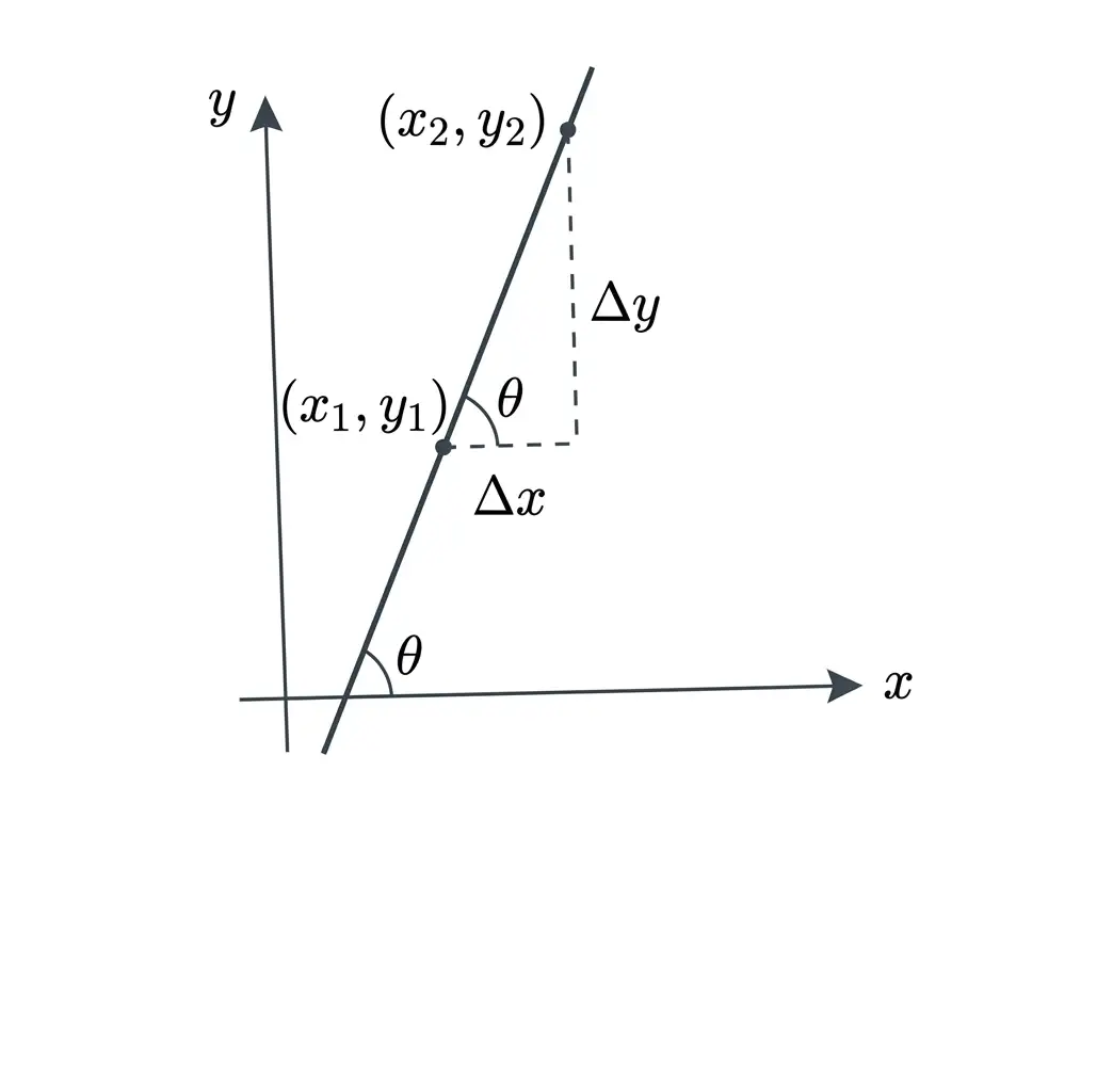
For points and , slope is the ratio of the coordinate changes.
If the line makes an angle with the positive -axis, its slope equals the tangent of that angle.
Finding Slope from Two Points
- Identify the two points as and .
- Find the horizontal and vertical changes using the same point order.
- Divide the vertical change by the horizontal change to obtain the slope.
A non-vertical straight line can be written with slope and -intercept .
| Type | Appearance | Slope |
|---|---|---|
| Positive | Rises from left to right | |
| Negative | Falls from left to right | |
| Zero | Horizontal line | |
| Undefined | Vertical line | , so the slope formula has a zero denominator |
Slopes of Parallel and Perpendicular Lines
| Relationship | Slope condition |
|---|---|
| Parallel lines | |
| Perpendicular lines |
Do not confuse a vertical line with a zero-slope line: horizontal lines have slope , while vertical lines have undefined slope.
What is the slope of the line through and ?
What is the condition for two non-vertical lines to be perpendicular?
Quick recap
- Coordinate geometry locates points on a plane using ordered pairs.
- Slope is vertical change divided by horizontal change: .
- The slope of a line at angle to the positive -axis is .
- A line in slope-intercept form is .
- Positive, negative, zero, and undefined slopes correspond to rising, falling, horizontal, and vertical lines.
- Parallel lines have equal slopes; perpendicular lines have slopes whose product is .
Tangent
Tangent
Tangent — A tangent is a line that touches a curve at exactly one point without crossing it.
- Circle: The tangent is perpendicular to the radius at the point of contact.
- At a point: Its slope gives the curve’s direction and instantaneous rate of change there.
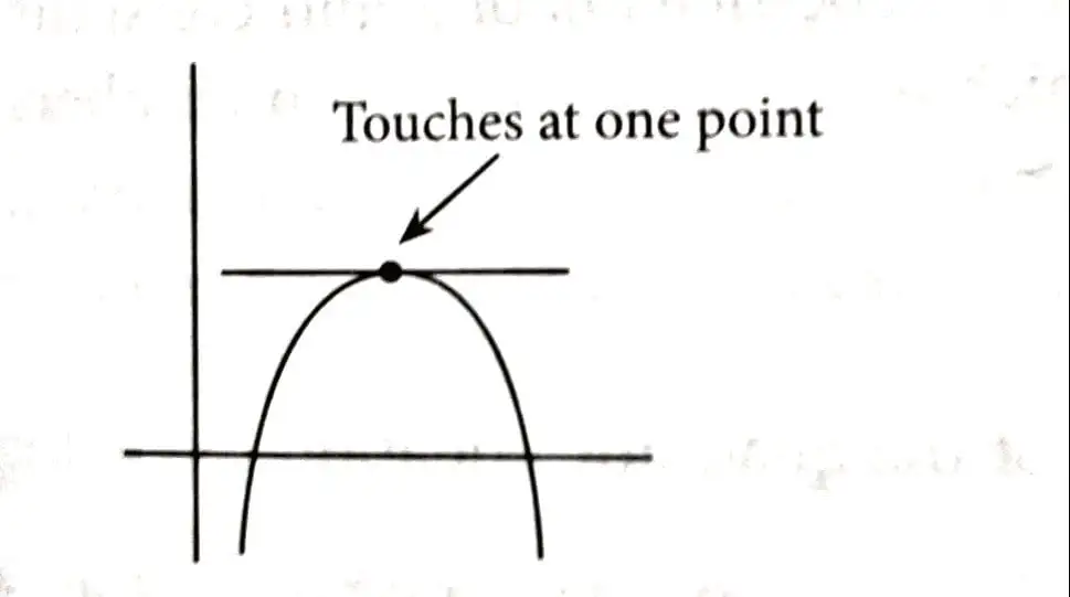
Slope of a Tangent
- Derivative: For a curve , the tangent slope at is the derivative evaluated at that point.
- Meaning: The derivative measures the instantaneous rate of change of with respect to .
Evaluate the derivative at the point of contact.
Secant
Secant — A secant is a line that intersects a curve at two or more points.
- Circle: A secant intersects a circle at two distinct points.
- Between two points: Its slope represents the average rate of change.
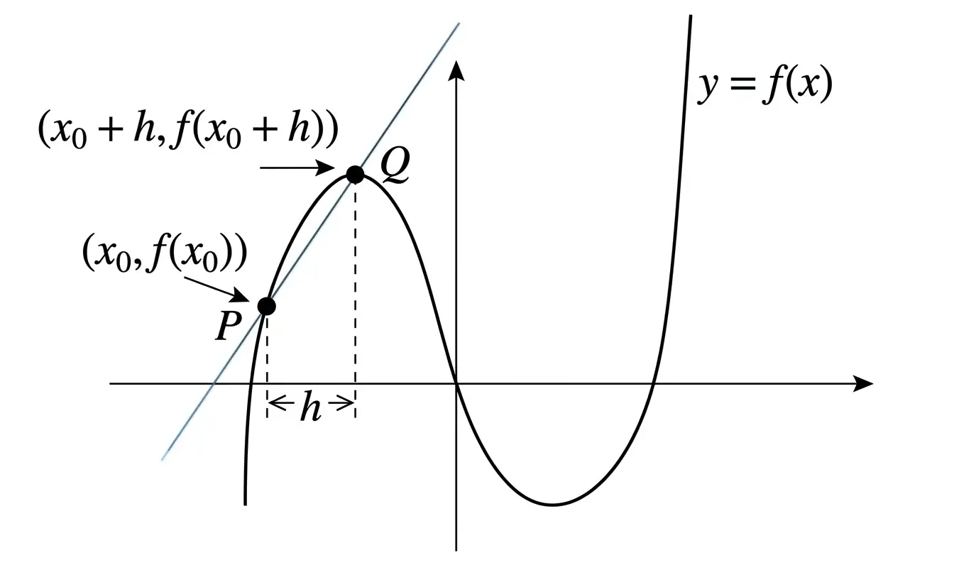
For points at and , the slope is the change in function values divided by the change in .
From Secant to Tangent
- Move the second point closer to by letting approach .
- The secant approaches the tangent as the two points merge.
- The limit of the secant slopes gives the derivative at (first principles).
At , the tangent slope is the limit of the secant slope as approaches .
| Feature | Tangent | Secant |
|---|---|---|
| Points involved | Touches a curve at one point | Intersects a curve at two or more points |
| Rate of change | Instantaneous | Average between two selected points |
| Slope | Derivative at a point | Change in function values divided by change in input |
Applications
- Coordinate geometry: Analyse geometric shapes and angles.
- Calculus: Solve problems involving motion and optimisation.
- Curve study: Understand properties of parabolas, ellipses and circles.
How is the tangent slope related to the secant slope?
Quick recap
- A tangent touches a curve at exactly one point; for a circle it is perpendicular to the radius at contact.
- For , the tangent slope at is .
- A secant intersects a curve at two or more points; for a circle it meets the circle at two distinct points.
- A secant slope gives average rate of change; a tangent slope gives instantaneous rate of change.
- The tangent slope is the limit of the secant slope as .
Co-ordinate Geometry
Straight Line
Here, is the slope and the constant term determines the -intercept.
Circle
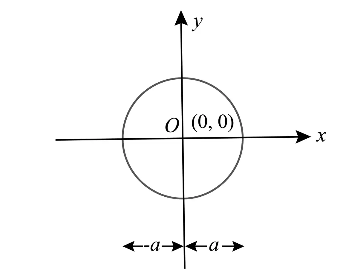
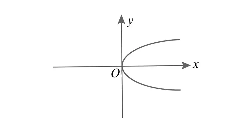
Parabola
The constant determines the curve's width.
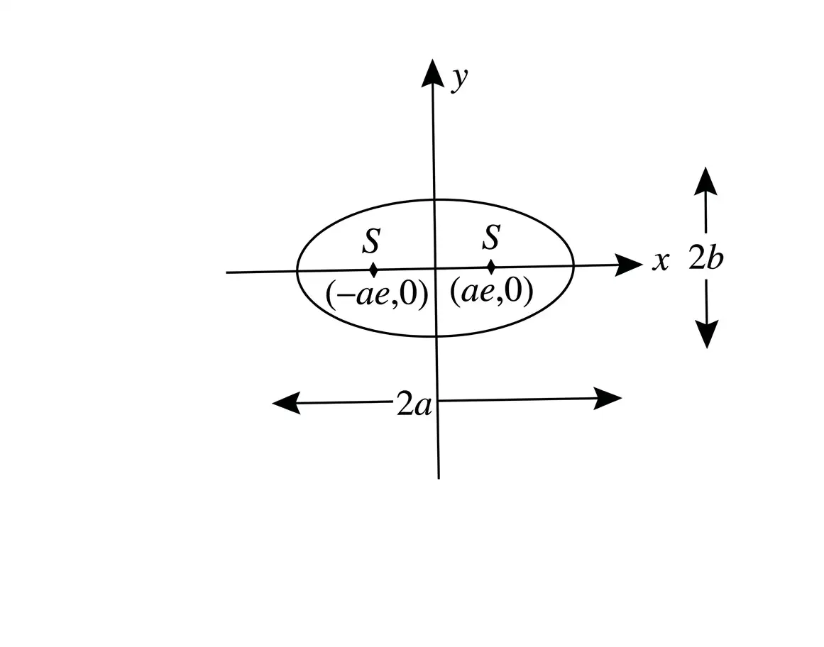
Ellipse
For the horizontal-major-axis form, .
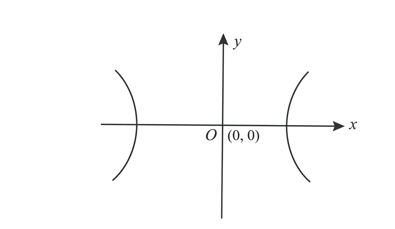
Hyperbola
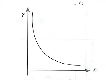
Rectangular Hyperbola
Here, is a constant.
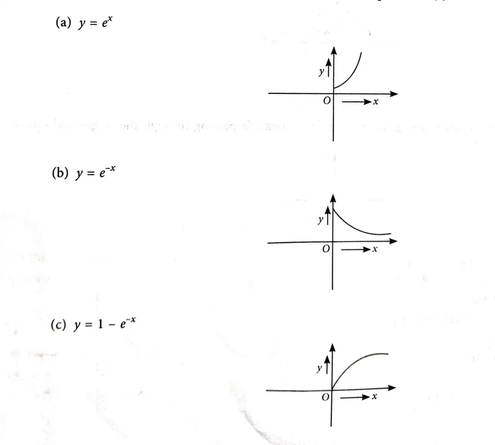
Exponential Graphs
State the equation, centre and radius of a circle centred at the origin.
Give the eccentricity and area of an ellipse with semi-axes and .
What relation defines a rectangular hyperbola?
Quick recap
- A straight line has slope ; check the sign of the constant when identifying its -intercept.
- A circle centred at the origin satisfies .
- The right-opening parabola through the origin is represented by .
- An ellipse has eccentricity less than , foci at in the standard orientation, and area .
- The standard hyperbola has opposite signs on its squared terms; a rectangular hyperbola satisfies .
- The common exponential graphs are , , and .
Trigonometry
Angle-Addition and Double-Angle Formulae-.
Use when the denominator is non-zero.
Sum-to-Product and Half-Angle Formulae
Standard-Angle Values
| Angle | |||||||||
|---|---|---|---|---|---|---|---|---|---|
| Radians | |||||||||
| Undefined |
Trigonometric Identities
| Use | Identities |
|---|---|
| Quotient and Pythagorean | ; ; ; |
| Complementary angles | ; ; |
| Negative angles | ; ; |
| Supplementary angles | ; ; |
| Shift by | ; ; |
| Shift by | ; ; |
| Periodicity | ; ; |
Inverse Trigonometric Formulae
Parity, reciprocals, and composition
- Odd/even relations: ; for ; for .
- Other inverse relations: ; for ; for .
- Composition: for ; only when .
- Reciprocal relations: for ; for .
- Positive reciprocal relation: for .
- Sum/difference: and when the principal-value branch permits; otherwise adjust by .
Inverse functions return principal values: in general, unless lies in the principal range.
Small-Angle Approximation and Series
Small-angle approximation — For angles close to zero, trigonometric functions can be estimated using simpler expressions; the angle must be measured in radians.
As , with in radians.
Angles are in radians; the series provide successively better approximations near .
Quick recap
- Use angle-addition identities to expand trigonometric functions of sums and differences.
- Double-angle, sum-to-product, and half-angle formulae connect common trigonometric expressions.
- Know the standard ratios at , , , , and and use symmetry for related angles.
- Apply the Pythagorean, complementary-angle, parity, shift, and periodicity identities carefully.
- Inverse-trigonometric functions have restricted domains and principal ranges; inverse composition is not unrestricted.
- For near zero, use small-angle approximations and series only with in radians.
Logarithm
Logarithm — If , then is the logarithm of to base , written as . It is the inverse operation of exponentiation.
Conditions and notation
- Base: and ; the logarithm's argument must be positive, .
- Meaning: is equivalent to .

Fundamental Properties of Logarithms
The logarithm of a product is the sum of the logarithms.
- Example: .
The logarithm of a quotient is the difference of the logarithms.
An exponent inside a logarithm becomes a multiplier.
Convert a logarithm to any valid base .
Switching the base and argument gives reciprocal logarithms.
Other Useful Results
These results follow directly from the definition of logarithms.
If , then:
With successive square roots inside the brackets, the nested logarithm evaluates to .
Characteristic and Mantissa
Characteristic — The integral part of a logarithm, when its decimal part is written positive, is called the characteristic.
Mantissa — The positive decimal part of a logarithm is called its mantissa.
Example
- For , the characteristic is and the mantissa is .
Antilogarithms
Antilogarithm — The number whose logarithm is is the antilogarithm of , written as .
Finding an antilogarithm from a table
- Separate the characteristic and mantissa of the given logarithm.
- Use the mantissa in the antilogarithm table; add the mean difference for any remaining digit.
- Place the decimal point using the characteristic. For a positive characteristic , the integral part has digits.
- Example: for , the table gives for and mean difference for the final digit; thus the table entry is and the required number is .
What are the characteristic and mantissa of ?
Quick recap
- A logarithm gives the exponent needed to raise a valid base to a given positive number.
- Product, quotient, and power rules convert logarithmic operations into sums, differences, and multipliers.
- Change-of-base and base-switch rules allow logarithms to be rewritten using other bases.
- , , and is undefined.
- The characteristic is the integral part; the mantissa is the positive decimal part.
- An antilogarithm table gives the mantissa digits; the characteristic determines the decimal placement.
Exponents
Meaning of Exponents
Exponent (power) — An exponent tells how many times the base is multiplied by itself.
Parts of a power
- Base: The number being repeatedly multiplied.
- Exponent: The number that indicates how many times the base is used as a factor.
- Example: .
Laws of Exponents
| Law | Rule | Key condition |
|---|---|---|
| Product of powers | Same base | |
| Quotient of powers | Same base; | |
| Zero exponent | ||
| Negative exponent | ||
| Power of a power | Multiply the exponents | |
| Power of a product | Applies to each factor | |
| Power of a quotient |
Do not add exponents when multiplying different bases: cannot generally be combined into one power.
Fractional Exponents
Fractional exponent — An exponent written as a fraction represents a root, a power, or both.
The denominator gives the root; the numerator gives the power.
Common fractional powers
- Square root: .
- Cube root: .
- Example: .
Decimal Exponents
Decimal exponent — A decimal exponent is an exponent written in decimal form; convert it to a fraction before applying exponent laws.
Example
- Convert: .
- Evaluate: .
Scientific Notation
Scientific notation — Scientific notation writes a number as a decimal coefficient multiplied by a power of .
For a non-zero number, choose the coefficient so that .
Example
- Large number: ; the decimal point moves places left.
Quick recap
- An exponent counts repeated multiplication of a base.
- For equal bases, multiply by adding exponents and divide by subtracting exponents.
- A zero exponent gives for a non-zero base; a negative exponent gives a reciprocal.
- In a fractional exponent, the denominator indicates the root and the numerator the power.
- Convert decimal exponents to fractions before evaluating.
- Scientific notation expresses a number as a coefficient times a power of .
Algebra
Algebraic Identities
These identities combine the squares of a sum and difference.
The first expression is a sum of squared pairwise differences; the second factors using the sum of the variables.
This factorisation is especially useful when the sum of the variables is zero.
Arithmetic Progression
Arithmetic mean (A.M.) — The A.M. of two numbers is their sum divided by ; it is the middle term when three numbers form an A.P.
For numbers and , the arithmetic mean is:
Geometric Progression
Geometric mean (G.M.) — The G.M. of two positive numbers is the non-negative square root of their product; it is the middle term when three numbers form a G.P.
For positive numbers and :
- A.M.–G.M. relation: For positive and , ; equality holds when .
Logarithm Laws
- Product and quotient: and .
- Power: .
- Change of base: , for valid logarithm bases and arguments.
Sums of Natural Numbers
| Sum | Formula |
|---|---|
| First powers | |
| Squares | |
| Cubes |
Binomial Expansions
- Binomial expansion: A power of a binomial can be expanded as a series whose coefficients depend on the exponent.
- Positive integer power: .
- Negative integer power: , for .
Exponential Expansion
Expansion of :
Logarithmic Expansion
Here, denotes the natural logarithm.
Quick recap
- Use the standard square, cube, and factorisation identities to simplify algebraic expressions.
- In an A.P., consecutive differences are constant; use and the A.P. sum formula.
- In a G.P., consecutive ratios are constant; use and the finite-sum formula.
- For positive numbers, the A.M. is at least the G.M., with equality when the numbers are equal.
- Logarithm laws turn products into sums, quotients into differences, and powers into coefficients.
- Remember the standard sums of , , and , and the conditions on the binomial and logarithmic series.
NEET Physics — ALL CHAPTERS
1
Basic Mathematics
2
Units and Measurement
3
Motion in a Straight Line
4
Motion in a Plane
5
Laws of Motion
6
Work, Energy and Power
7
System of Particles and Rotational Motion
8
Gravitation
9
Mechanical Properties of Solids
10
Mechanical Properties of Fluids
11
Thermal Properties of Matter
12
Thermodynamics
13
Kinetic Theory
14
Oscillations
15
Waves
16
Electric Charges and Fields
17
Electrostatic Potential and Capacitance
18
Current Electricity
19
Moving Charges and Magnetism
20
Magnetism and Matter
21
Electromagnetic Induction
22
Alternating Current
23
Electromagnetic Waves
24
Ray Optics and Optical Instruments
25
Wave Optics
26
Dual Nature of Radiation and Matter
27
Atoms
28
Nuclei
29
Semiconductor Electronics: Materials, Devices and Simple Circuits