NEET UG . NEET Physics . Physics . Current Electricity
Chapter 18: Current Electricity
Ch 18
NEET Physics
NEET UG
Electric Current
Charges in Motion
Steady and Unsteady Charge Flow
- Electric current occurs when electric charges move.
- Unsteady flow: In lightning, charge flows from a cloud to Earth through the atmosphere, but the flow is not steady.
- Steady flow: Charges flow steadily in devices such as a torch and a cell-driven clock.
Definition and Measurement of Electric Current
Electric current — The rate at which electric charge passes through a cross-section of a conductor is called electric current.
Current in Steady and Changing Flow
- Steady current: The charge passing per unit time remains constant; for charge crossing in time , .
- Electron flow: If free electrons cross the section in time , their total charge magnitude is , where is the magnitude of the charge of one electron.
- Changing current: For a non-steady current, the current at an instant is the rate of change of charge, .
Use when the current is steady; electrons cross a conductor's cross-section in time .
Use when the current varies with time.
SI Unit
- Unit: The SI unit of electric current is the ampere, symbol .
- Definition of ampere: ; one ampere means one coulomb of charge flows per second.
Define electric current and state its SI unit.
Quick recap
- Electric current is charge flowing through a conductor.
- Current is the rate of charge flow across a conductor's cross-section.
- For steady current, .
- For changing current, instantaneous current is .
- The SI unit is the ampere: .
- Lightning is an example of unsteady charge flow; a torch is an example of steady flow.
Electric Currents in Conductors
Electron Motion in a Conductor
Here, is the magnitude of electron charge, is electric-field strength and is electron mass. The acceleration is opposite to the field direction.
Drift and Current in a Conductor
How Current Is Established
- Electric field: Charges and at opposite ends of a metallic conductor create an electric field from the positive end to the negative end.
- Electron drift: Free electrons move opposite to the field, giving rise to electric current.
- Steady current: A continuous supply of charge at the conductor’s ends maintains the field and hence a steady current; cells or batteries provide this supply.
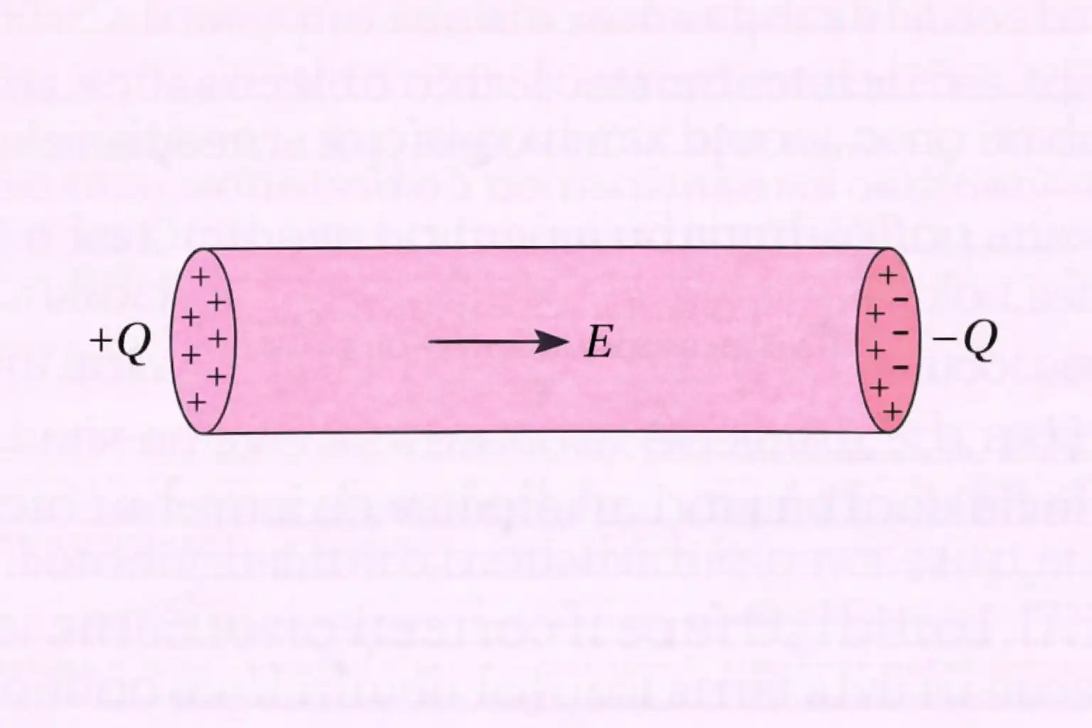
Do not confuse electron drift with the electric-field direction: electrons move opposite to the field.
Why does an electron not keep accelerating indefinitely in a conductor?
Quick recap
- Metal electrons move randomly when no electric field is applied.
- An electric field accelerates electrons opposite to its direction.
- Collisions continually interrupt the electrons’ acceleration.
- A field between opposite charges causes electron drift and current.
- Cells or batteries maintain a continuous charge supply for steady current.
Ohm’s Law
Ohm’s Law
- Ohm’s law: For a conductor under suitable conditions, the potential difference across it is directly proportional to the current through it.
- Equation: , where is the resistance of the conductor.
- Resistance: For a uniform conductor, ; it depends on the material and dimensions of the conductor.
Quick recap
- Ohm’s law gives when physical conditions are fixed.
- Resistance depends on the conductor’s material, length and cross-sectional area.
- Resistivity is a material-dependent constant independent of the conductor’s dimensions: .
- Doubling length or halving cross-sectional area doubles resistance, all else unchanged.
- Current density is and the potential difference in a uniform field is .
- The equivalent field form is , where .
The Origin of Resistivity and Drift of Electrons
Drift Velocity and Relaxation Time
Drift velocity — The average velocity acquired by charge carriers in a conductor due to an applied electric field is called drift velocity.
Electron motion in a conductor
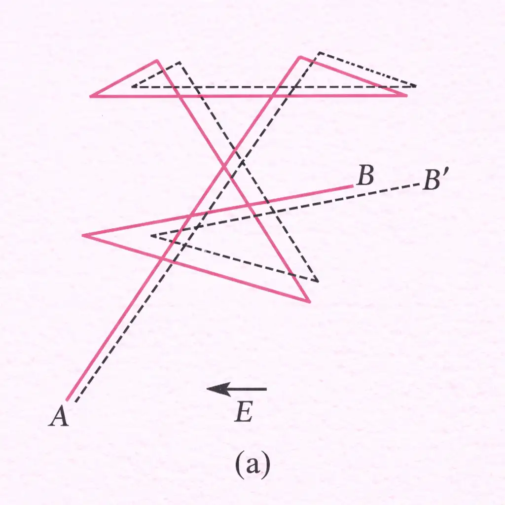
- Random motion: Without an electric field, electrons move randomly, so their average motion through the conductor is zero.
- Drift: An applied electric field produces a small net motion of electrons opposite to the field; conventional current is in the field’s direction.
- Collisions: Collisions interrupt electron acceleration; the average time between successive collisions is the relaxation time, .
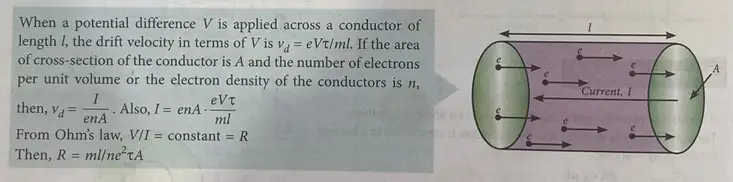
These are magnitudes; an electron’s force and acceleration are opposite to the electric field.
The drift-speed magnitude acquired over the average time between collisions is given below.
For a uniform field along a conductor of length and potential difference , .
Current and Drift Velocity
Number of charge carriers
- Volume: A conductor segment of length and cross-sectional area has volume .
- Total electrons: If is the number of free electrons per unit volume, the segment contains electrons.
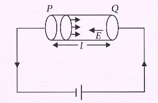
In time , all electrons in the segment pass a cross-section. Each electron has charge magnitude .
Current Density and Conductivity
Current density — The magnitude of current per unit cross-sectional area is the current density, .
For electrons of number density , current density is related to drift velocity and electric field as shown.
Conductivity relates current density to electric field by .
Mobility and Charge Carriers
Mobility — Mobility is the magnitude of drift velocity per unit magnitude of the applied electric field.
The SI unit of mobility is ; a practical unit is .
| Material | Mobile charge carriers |
|---|---|
| Metals | Free electrons |
| Ionised gases | Electrons and positively charged ions |
| Electrolytes | Positive and negative ions |
| Semiconductors | Electrons and holes (electron vacancies) |
In semiconductors, and are the electron and hole concentrations, respectively; and are their relaxation times, and and their respective masses.
Do not confuse electron drift direction with conventional current: electrons drift opposite to the electric field, while conventional current points along it.
Derive the relation between current and drift velocity.
Write the expressions for conductivity and current density in the electron model.
Quick recap
- Electrons move randomly without a field and acquire a net drift opposite to the electric field when it is applied.
- Relaxation time is the average time between successive collisions.
- The force and acceleration magnitudes are and ; drift speed is .
- For a conductor segment, and .
- Current density is , with .
- Mobility is ; in semiconductors, and denote electron and hole concentrations.
Limitations of Ohm’s Law
Ohm’s Law Is Not Universal
- Scope: Ohm’s law is a commonly observed property under suitable conditions, not a universal law of nature.
- Non-ohmic conductors: Some circuit elements have a nonlinear relationship between voltage and current.
Resistance Changes as a Conductor Heats
- Heating effect: As current increases, a conductor can heat up and its resistance can rise, making the voltage–current relationship nonlinear.
Voltage Polarity Can Affect Current
- Polarity dependence: In a diode, reversing the voltage while keeping its magnitude the same may not produce an equal current in the opposite direction.
More Than One Voltage for the Same Current
Why is Ohm’s law not applicable to every circuit element?
What is meant by a non-unique – relation? Give an example.
Quick recap
- Ohm’s law is a common property under suitable conditions, not a fundamental law of nature.
- Non-ohmic elements have nonlinear voltage–current relations.
- Heating from increased current can raise a conductor’s resistance.
- A diode’s current response can differ for equal voltages of opposite polarity.
- In GaAs, the same current can correspond to multiple voltages; its curve can have a negative-resistance region.
Resistivity of Various Materials
Resistivity Across Materials
- Material range: Materials are broadly classified by resistivity as conductors, semiconductors and insulators.
- Comparison: Metals have low resistivity, insulators have very high resistivity, and semiconductors lie between them.
Semiconductors and Impurities
- Temperature: Semiconductor resistivity decreases as temperature rises.
- Reason: Heating frees more electrons, increasing the number density of charge carriers.
- Impurities: Adding a small amount of suitable impurity can reduce a semiconductor’s resistivity.
- Use: This control of resistivity is used in making electronic devices.
Quick recap
- Metals have low resistivity: to .
- Insulators such as ceramic, rubber and plastics have resistivities about times greater than metals or more.
- Semiconductors have resistivities between those of metals and insulators.
- Semiconductor resistivity decreases as temperature increases.
- Small amounts of suitable impurities can lower semiconductor resistivity, enabling electronic-device applications.
Temperature Dependence of Resistivity
Temperature Dependence in Metals
Temperature coefficient relation — For a small temperature range, a conductor’s resistivity varies approximately linearly with temperature relative to a reference temperature.
Here, is resistivity at reference temperature , and is the temperature coefficient of resistivity.
Why metal resistivity increases
- Free-electron density: In metals, the number density of free electrons is approximately fixed as temperature rises.
- Lattice vibrations: Metal ions vibrate more strongly at higher temperature, causing more frequent electron collisions.
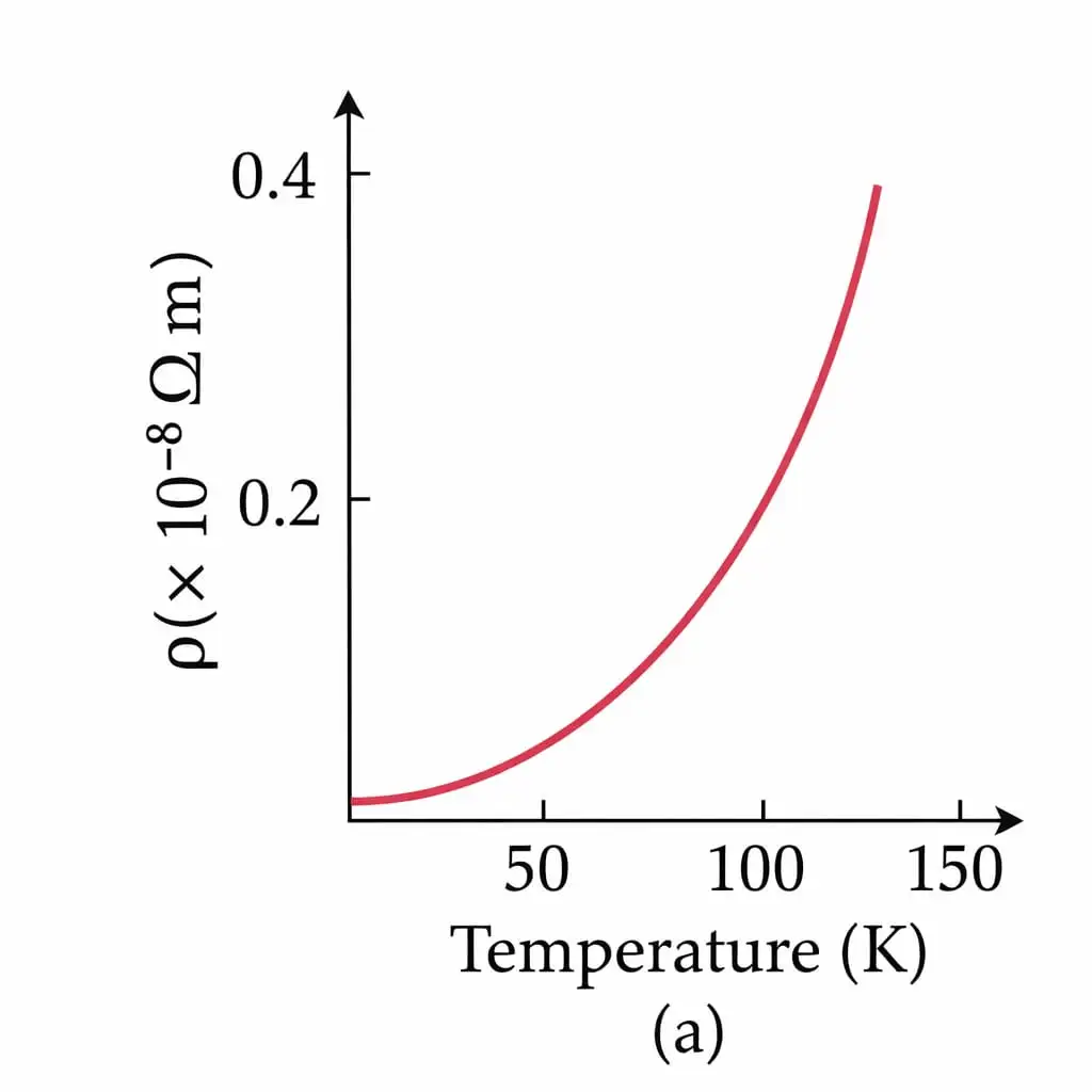
- Relaxation time: More frequent collisions reduce the relaxation time . Since , resistivity increases as decreases.
- Result: Metal resistance increases with temperature; the rise in resistivity is generally nonlinear over a wide temperature range.
Alloys and Temperature
- Weak dependence: Alloy resistivity changes only slightly with temperature; nichrome is an example.
- Nearly temperature-independent: Manganin’s resistivity is almost independent of temperature, so it is used to make standard resistors in meter bridges and potentiometers.
- At absolute zero: Pure metals have very small resistivity, whereas alloys retain residual resistivity.
Temperature Dependence in Semiconductors
- Trend: Semiconductor resistivity decreases rapidly as temperature increases.
- Cause: Heating frees more electrons, increasing the free-electron number density .
- Key factor: In semiconductors, the change in is the dominant effect; unlike metals, the temperature trend is not mainly governed by a decrease in relaxation time .
| Material | Resistivity as temperature rises | Main reason / example |
|---|---|---|
| Metals | Increases | is nearly fixed; stronger lattice vibrations reduce . |
| Alloys | Changes weakly; manganin is nearly independent | Nichrome shows weak dependence; manganin is used for standard resistors. |
| Semiconductors | Decreases rapidly | Heating increases the number density of free electrons. |
Why does the resistivity of a metal increase when heated?
Why is manganin suitable for standard resistors?
Quick recap
- For a limited temperature range, .
- In metals, heating increases lattice vibrations, reduces , and raises resistivity.
- Metal resistivity generally rises nonlinearly over a wide temperature range.
- Alloys have weak temperature dependence; manganin is nearly temperature-independent and useful in standard resistors.
- At absolute zero, pure metals have very small resistivity, while alloys retain residual resistivity.
- Semiconductor resistivity falls rapidly on heating because the free-electron density increases.
Electrical Energy, Power
Electrical Energy and Power
Using Ohm’s law, power may be written in three equivalent forms.
Power Transmission
For delivered power and cable resistance , use .
Resistors in Series and Parallel
| Point | Series | Parallel |
|---|---|---|
| Connection | Resistors are joined end to end. | Each resistor connects across the same two points. |
| Current and voltage | Same current passes through every resistor; voltage divides. | Same voltage is across every branch; current divides among branches. |
| Equivalent resistance | ||
| For three resistors |
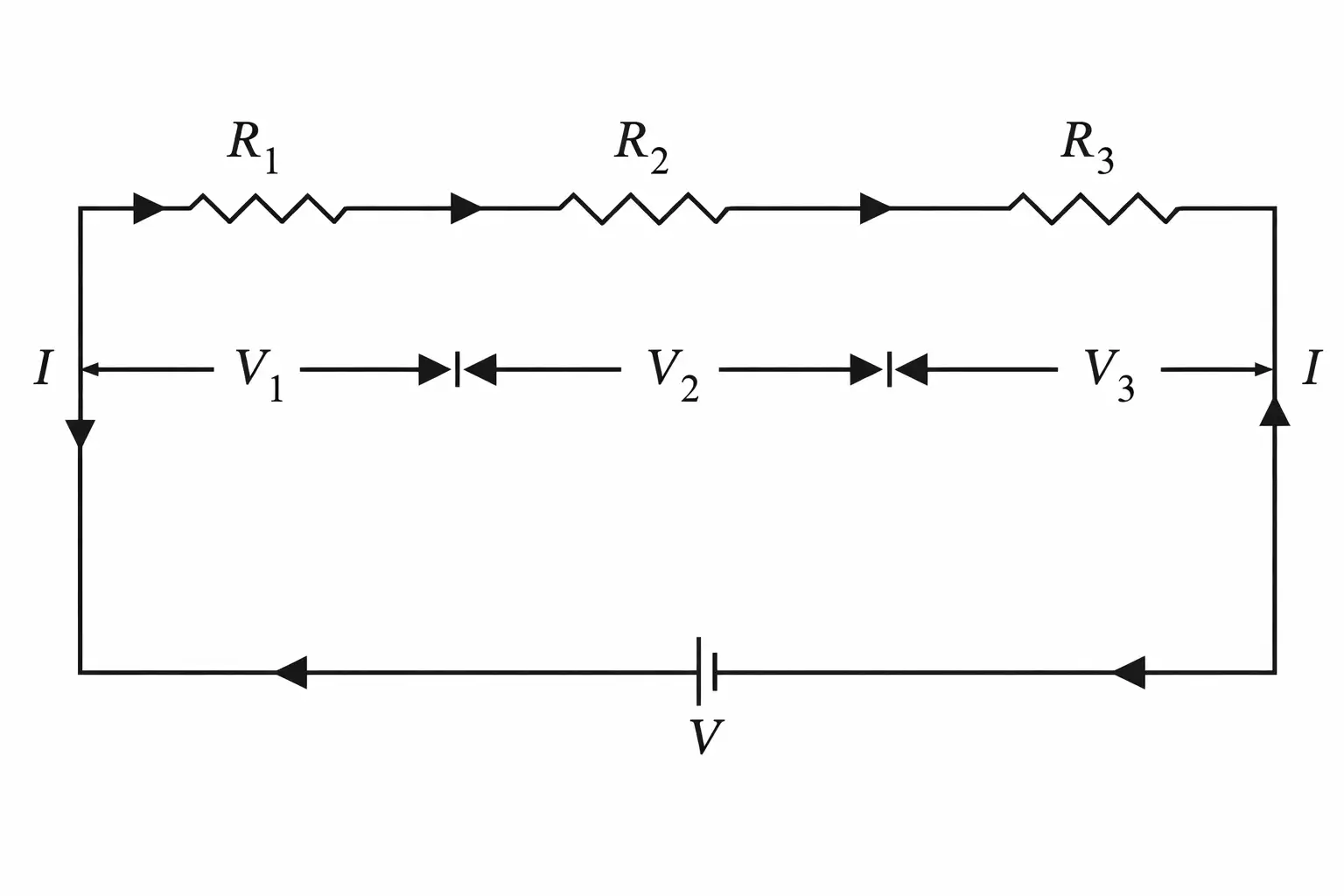
For each resistor, apply Ohm’s law; the total voltage is the sum of the drops.
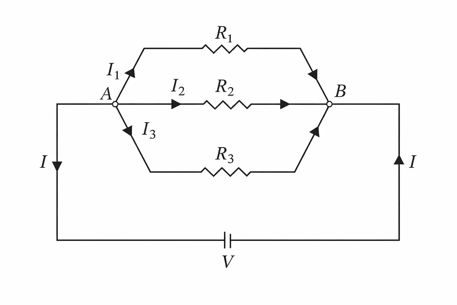
The main current is the sum of branch currents; each branch obeys Ohm’s law.
Do not mix up the rules: series has the same current; parallel has the same voltage.
Circuit Simplification by Symmetry
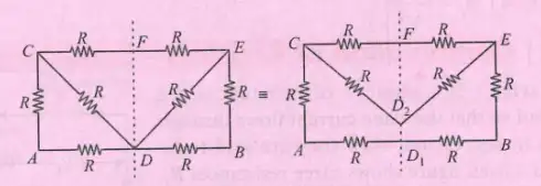
Delta–Star Transformation
Each star resistance equals the product of the corresponding two delta resistances divided by the sum of all three delta resistances.
Equipotential Points: Worked Network
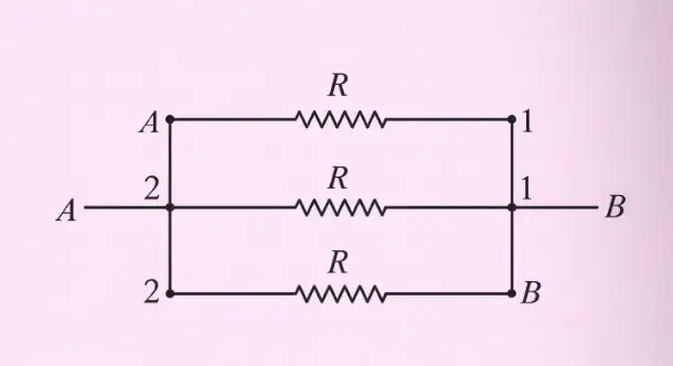
For three identical resistors, the equivalent resistance is one-third of a single resistance.
Quick recap
- Charge transferred in time is ; electrical energy is .
- Power dissipated is .
- Transmission loss is ; for fixed delivered power, higher voltage means lower current and less loss.
- Series resistances add; the same current passes through each resistor.
- Parallel reciprocals add; every branch has the same voltage.
- Symmetry and equipotential nodes allow networks to be redrawn and simplified.
- For three equal resistors in parallel, .
Cells,Emf,Internal Resistance
Electrochemical Cell and EMF
- Electrochemical cell: It converts chemical energy into electrical energy and acts as a source of direct current.
- EMF: The emf of a cell is the potential difference across its terminals when no current flows, that is, in an open circuit.
Internal Resistance and Terminal Voltage
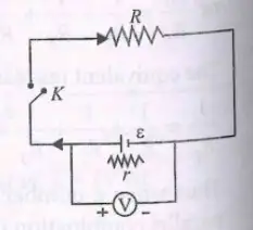
Charging a Cell
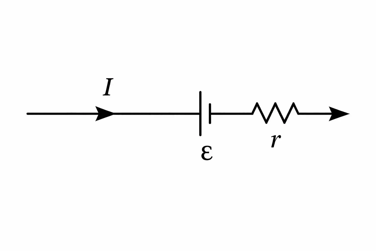
| Mode | Terminal voltage |
|---|---|
| Discharging | ; less than emf |
| Charging | ; greater than emf |
- In the terminal-voltage equations, is current and is the cell’s internal resistance.
- The sign of depends on whether the cell is discharging or charging.
Quick recap
- An electrochemical cell converts chemical energy into electrical energy and supplies DC.
- EMF is the terminal potential difference when the cell is open-circuited and no current flows.
- Internal resistance is the opposition to current inside the cell.
- Internal resistance depends on electrode area and spacing, and the electrolyte’s nature, temperature and concentration.
- During discharge, ; during charging, .
Cells in Series and in Parallel
Cells in Series
Equivalent circuit
- Series grouping connects identical cells one after another; their emfs and internal resistances add.
- Net values are emf and internal resistance ; the external resistance remains .
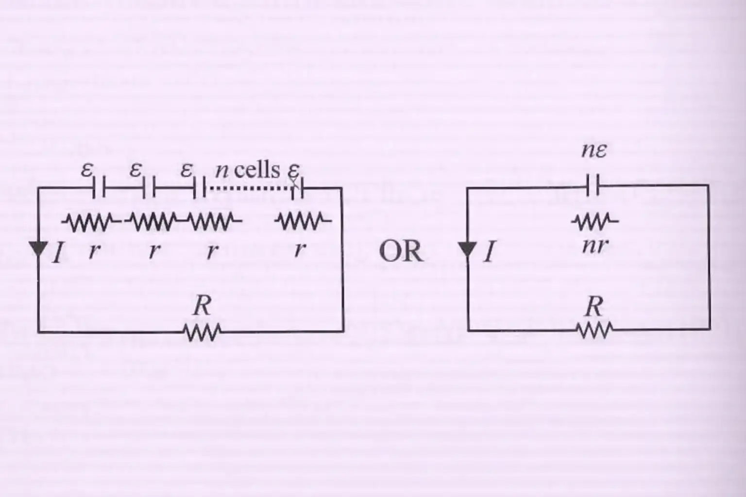
Use the total circuit resistance, including the cells’ internal resistance.
Cells in Parallel
Identical cells
- Parallel grouping connects like terminals together. For identical cells, the equivalent emf stays .
- Equivalent internal resistance is ; the external resistance is .
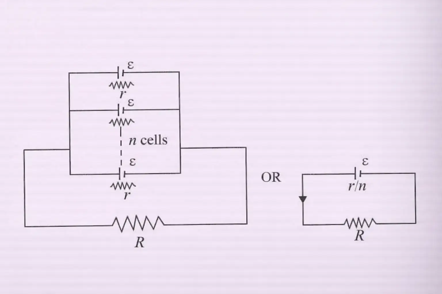
The current can also be written by multiplying numerator and denominator by .
Cells with different emfs
- Unequal cells in parallel: for two cells with emfs and internal resistances , use the equivalent quantities below.
- Connection: the cells are connected in parallel with the same polarity.
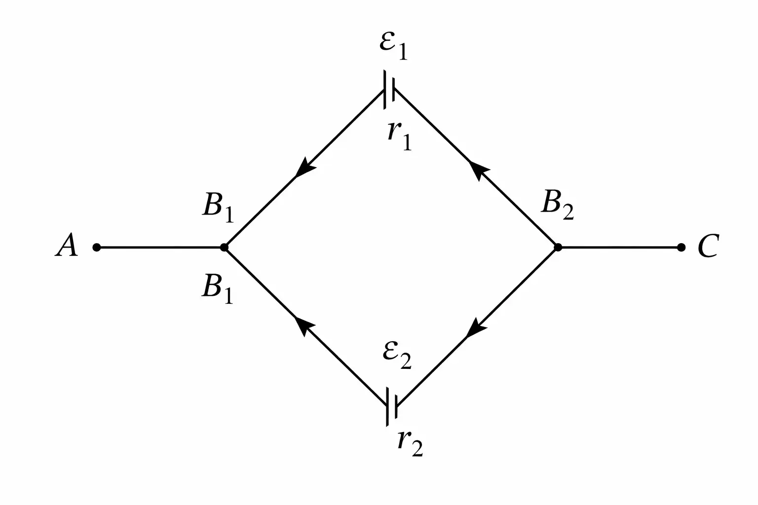
For cells connected with the same polarity:
This is the parallel combination of the two internal resistances.
Mixed Grouping of Cells
Series rows connected in parallel
- Arrangement: each row has identical cells in series, and such rows are connected in parallel.
- Equivalent values: emf is and internal resistance is ; the external resistance is .
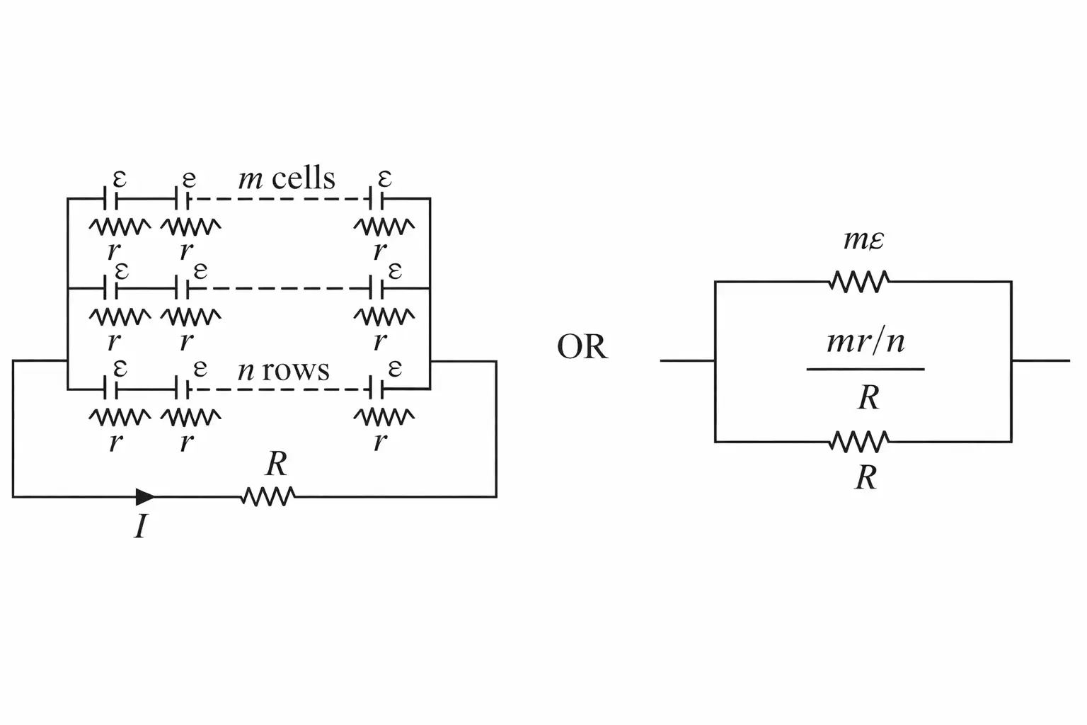
Use total emf and total internal resistance .
What are the equivalent emf and internal resistance of identical cells in series and in parallel?
Give the equivalent emf and internal resistance for two unequal cells connected in parallel with the same polarity.
Quick recap
- In series, cell emfs and internal resistances add: and .
- For series cells, .
- For identical parallel cells, emf stays and internal resistance becomes .
- For two unequal cells in parallel, and .
- For cells per series row and parallel rows, emf is and internal resistance is .
- Circuit current is equivalent emf divided by the sum of external and equivalent internal resistance.
Kirchhoff’s Rules
Kirchhoff’s Rules for Circuits: the Junction and Loop Rules apply even when resistors are not in series or parallel.
Junction rule (Kirchhoff’s current law) — At any junction, the total current entering equals the total current leaving; this follows from conservation of charge.
Applying the junction rule
- Signed form: Choose entering or leaving currents as positive consistently; the algebraic sum of currents at a junction is zero.
- Example: For the shown junction, .
- Meaning: Charge does not accumulate at an ideal junction.
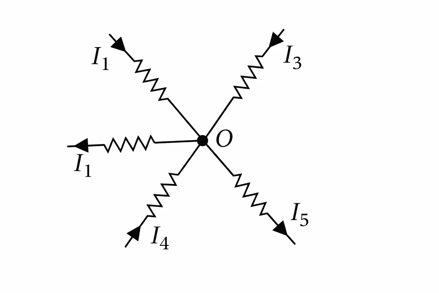
Loop rule (Kirchhoff’s voltage law) — Around any closed loop, the algebraic sum of potential rises and drops is zero; this follows from conservation of energy.
Applying the loop rule
- Sign convention: Add a potential rise and subtract a potential drop, or use the opposite convention consistently.
- Example: The signed voltage changes in the illustrated loop satisfy .
- Generality: A loop may contain resistors, batteries, or other linear or nonlinear circuit elements.
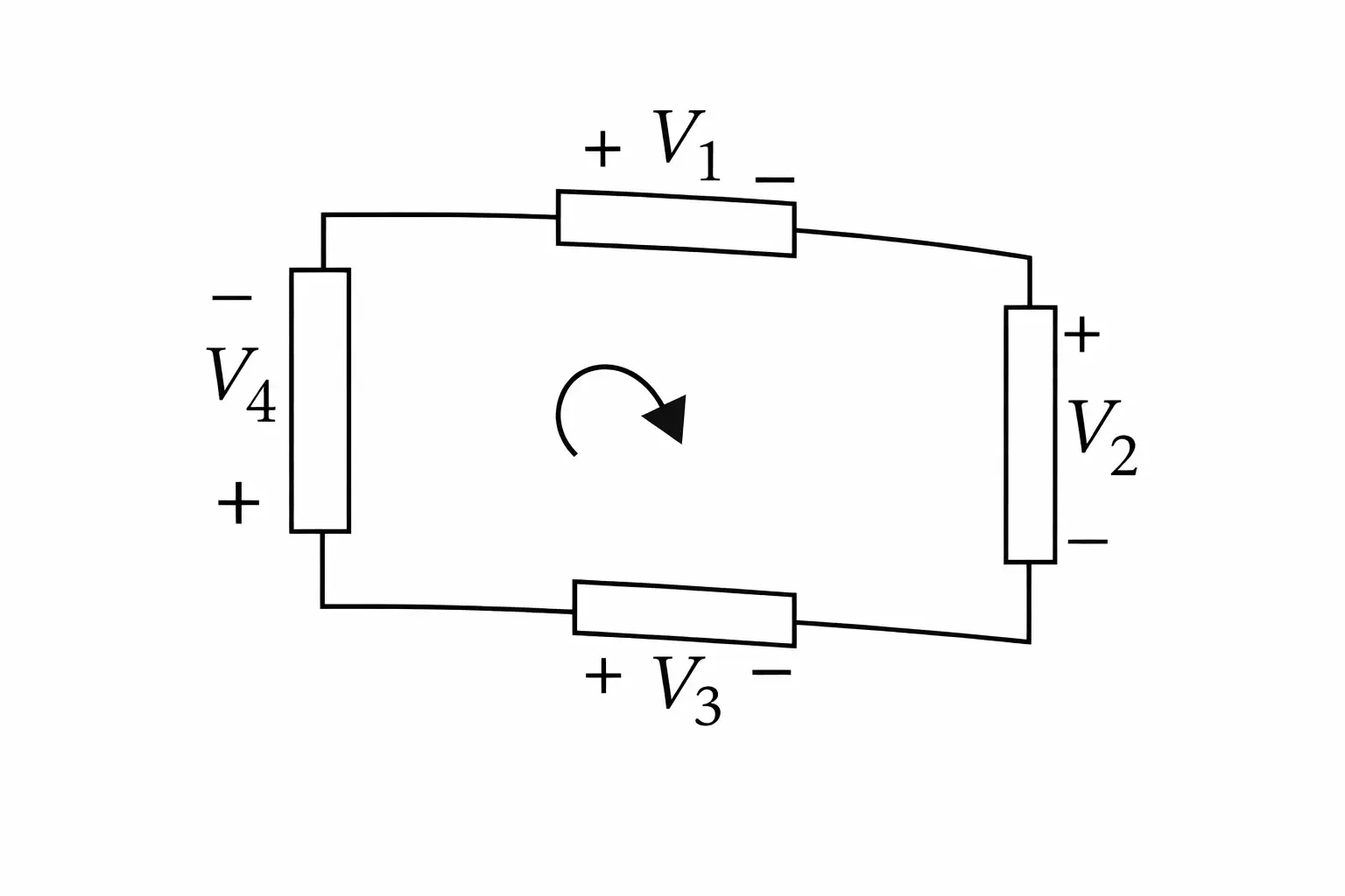
Solving a circuit using Kirchhoff’s rules
- Assign a direction to the current in every branch; any initial choice is valid.
- Mark resistor polarities consistently with the chosen current direction. Outside a battery, conventional current flows from higher to lower potential.
- Apply the junction and loop rules to obtain as many independent equations as there are unknowns.
- Solve the equations simultaneously; a negative current means its actual direction is opposite to the assumed direction.
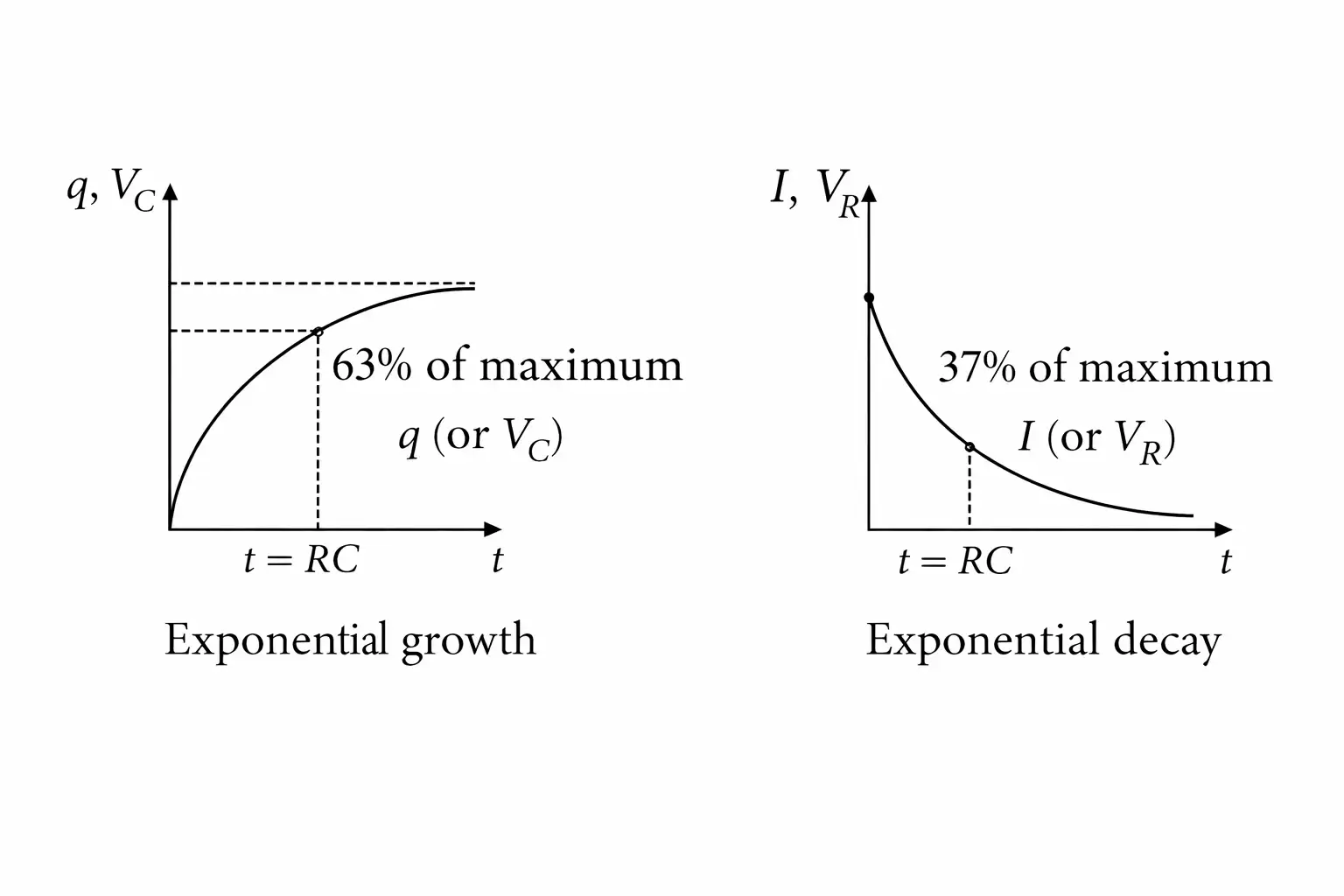
Charging of a Capacitor: In a series RC circuit connected to a source, charge builds up while current decays.
Charging behaviour
- Charge: increases from zero toward its maximum .
- Current: It is initially maximum and decreases exponentially as the capacitor charges.
- Voltages: The source voltage is shared by the capacitor and resistor: . As rises, and current fall.
- Time constant: sets the characteristic timescale of charging and discharging.
For a source voltage , the charge approaches .
The initial current is .
Discharging of a Capacitor: A charged capacitor releases charge through a resistor, with circuit quantities decaying exponentially.
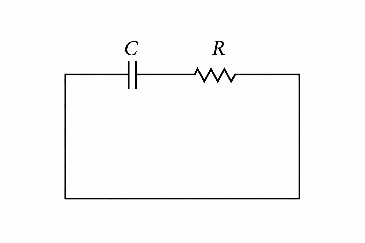
The initial charge is , where is the capacitor’s initial voltage.
With the current sign chosen in the direction of charging, the discharge current is negative; its magnitude starts at .
Discharging behaviour
- Voltage relation: With signed potential changes around the loop, ; the capacitor and resistor voltage magnitudes are equal.
- Decay: Charge, capacitor voltage, resistor voltage, and current magnitude all decrease exponentially.
- Time constant: At , a decaying quantity falls to about of its initial value (a decrease).
- DC behaviour: In a DC circuit, current falls to zero after the charging or discharging transient; a capacitor then blocks steady current.
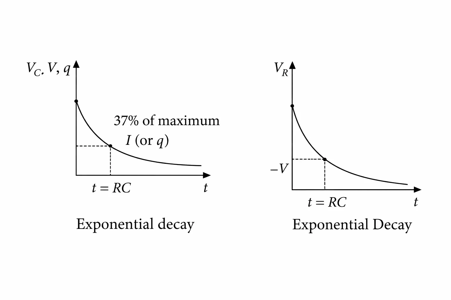
Effect of the time constant
- Small : Circuit quantities change rapidly at the start because the time constant is short.
- Large : The charging or discharging process takes longer.
State Kirchhoff’s junction and loop rules and the conservation principle behind each.
What is the time constant of a series RC circuit, and what happens at ?
Write the charge and current equations for a charging capacitor.
Quick recap
- Kirchhoff’s junction rule expresses conservation of charge: current entering equals current leaving.
- Kirchhoff’s loop rule expresses conservation of energy: signed potential changes around a closed loop sum to zero.
- Assume branch-current directions consistently; a negative answer indicates the true direction is opposite.
- For charging, and .
- For discharging, and the current magnitude decays exponentially.
- The RC time constant is ; at , charging reaches about and decaying quantities remain at about .
Wheatstone Bridge
Balanced Wheatstone Bridge
Wheatstone bridge — An arrangement of four resistors that can determine one unknown resistance when the other three are known.
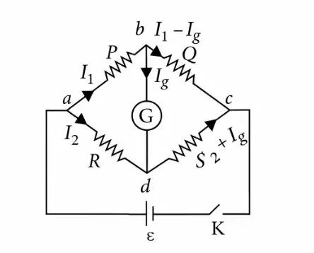
Balance condition
- Balance: The bridge is balanced when no current flows through the galvanometer: .
- At balance: The two loop relations give and .
- Resistance relation: Dividing the loop relations gives .
- Unknown resistance: Rearrange the balance relation; for example, if is unknown, .
Use when the galvanometer current is zero.
Meter Bridge
Meter bridge — A practical form of Wheatstone bridge used to measure an unknown resistance using a one-metre wire.
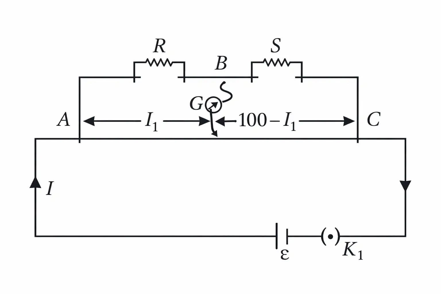
Principle and balance
- Principle: At the null point, the meter bridge satisfies the Wheatstone-bridge balance condition.
- Wire lengths: If the balance point is at length from one end, the two wire segments have lengths and cm.
- Balance point: Choose the known resistance so the null point lies as close as possible to the centre of the wire.
For resistance in the first gap and in the second gap, with balance length measured in centimetres.
Potentiometer
Potentiometer — An instrument that measures or compares potential differences by balancing them against the potential drop along a wire.
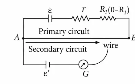
Principle and circuit
- Principle: With a uniform wire and constant current, the potential drop across a portion is directly proportional to its length.
- Potential gradient: is the potential drop per unit length; a length has a drop .
- Wire requirements: The potentiometer wire must have uniform cross-section and high resistance; current through it must remain constant.
- Primary circuit: Contains the constant-voltage driving source, rheostat, resistance box and potentiometer wire.
- Secondary circuit: Contains the unknown circuit or source being tested and a galvanometer.
Here, is the potential gradient.
Applications of a Potentiometer
Comparing the EMFs of two cells
- Cell 1: Connect only the first cell; if its balance length is , then .
- Cell 2: Connect only the second cell; if its balance length is , then .
- Comparison: The same potential gradient applies to both measurements, so the EMF ratio equals the balance-length ratio.
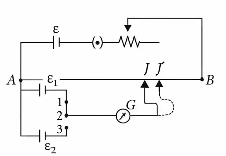
Use the balance lengths measured for the two cells.
Determining a cell’s internal resistance
- Key open: With no current drawn from the cell, its EMF balances at length : .
- Key closed: Connect a known resistance across the cell; its terminal potential difference balances at length : .
- Relation: The cell supplies current through , so .
- Result: Substituting the balance lengths gives the internal resistance.
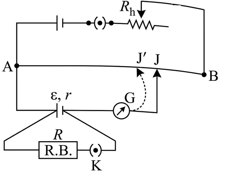
Here, is the external resistance connected across the cell.
Driving-cell and polarity conditions
- Driving EMF: It must exceed each EMF being compared: and .
- Series combination: To compare the sum of two EMFs, require .
- Polarity: Connect the positive terminal of the test cell (or combination) to the potentiometer-wire end connected to the driving cell’s positive terminal.
State the balance condition for a Wheatstone bridge.
How are the EMFs of two cells compared using a potentiometer?
Write the potentiometer formula for a cell’s internal resistance.
Quick recap
- A Wheatstone bridge is balanced when , giving .
- A meter bridge applies the Wheatstone-bridge balance principle to a one-metre wire.
- In a uniform potentiometer wire carrying constant current, .
- The ratio of two cell EMFs equals the ratio of their balance lengths.
- A cell’s internal resistance is .
- The driving EMF must be greater than the EMF or combined EMFs being compared, and the test-cell polarity must match the driving-cell end.
NEET Physics — ALL CHAPTERS
1
Basic Mathematics
2
Units and Measurement
3
Motion in a Straight Line
4
Motion in a Plane
5
Laws of Motion
6
Work, Energy and Power
7
System of Particles and Rotational Motion
8
Gravitation
9
Mechanical Properties of Solids
10
Mechanical Properties of Fluids
11
Thermal Properties of Matter
12
Thermodynamics
13
Kinetic Theory
14
Oscillations
15
Waves
16
Electric Charges and Fields
17
Electrostatic Potential and Capacitance
18
Current Electricity
19
Moving Charges and Magnetism
20
Magnetism and Matter
21
Electromagnetic Induction
22
Alternating Current
23
Electromagnetic Waves
24
Ray Optics and Optical Instruments
25
Wave Optics
26
Dual Nature of Radiation and Matter
27
Atoms
28
Nuclei
29
Semiconductor Electronics: Materials, Devices and Simple Circuits