NEET UG . NEET Physics . Physics . Motion in a Straight Line
Chapter 3: Motion in a Straight Line
Ch 3
NEET Physics
NEET UG
Instantaneous Velocity and Speed
Describing Motion
Rectilinear motion — Motion along a straight line.
Path Length and Displacement
Distance (path length) — The length of the actual path travelled between an object's initial and final positions.
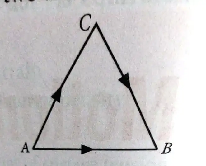
Displacement — The change in position from the initial point to the final point, in a specified direction; it is the straight-line vector from start to finish.
| Point | Distance | Displacement |
|---|---|---|
| Meaning | Length of the actual path | Change in position from start to finish |
| Quantity | Scalar; non-negative | Vector; may be positive, negative or zero in one dimension |
| Path dependence | Depends on the route travelled | Depends only on initial and final positions |
| Magnitude | Always at least as large as displacement magnitude | Shortest separation between the endpoints |
Position–Time Graphs
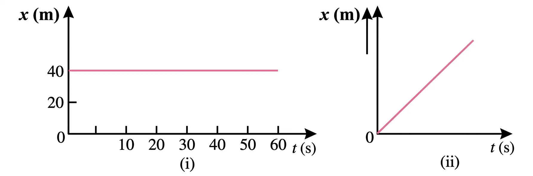
- Use: A position–time graph represents motion and helps analyse how position changes with time.
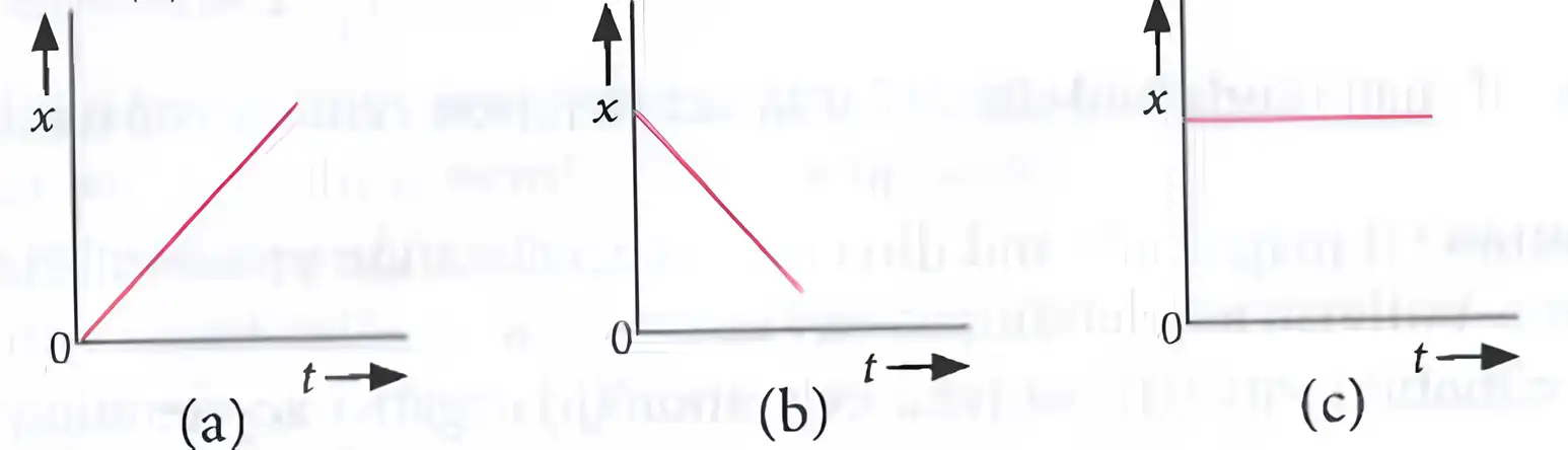
- Uniform motion: Equal distances are covered in equal time intervals; the position–time graph is a straight line.
- At rest: Position remains constant, so the graph is horizontal.
Average Velocity and Average Speed
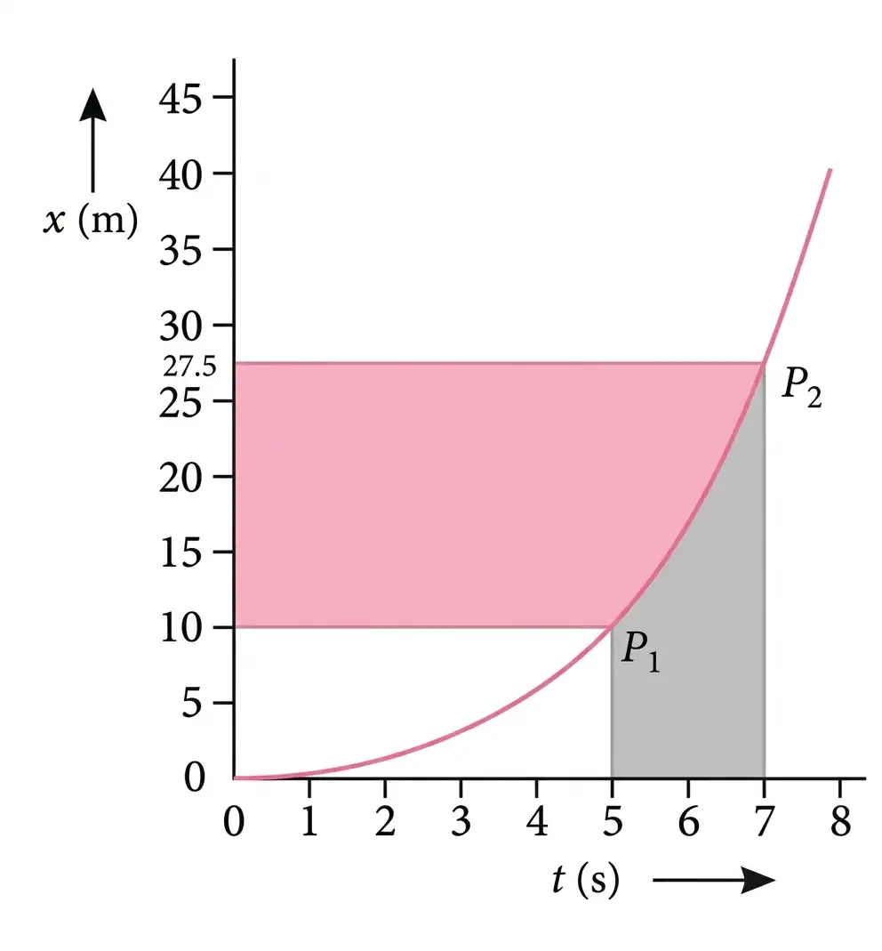
Average velocity — Displacement divided by the time interval in which it occurs.
Here, and are positions at times and , respectively.
- Example: From to , position changes from to ; average velocity is .
Average speed — The total path length travelled divided by the total time taken.
Use the first form when distances are given with their speeds, and the second when speeds and their time intervals are given.
Do not assume average speed equals average velocity for every straight-line journey. If direction reverses, distance exceeds the magnitude of displacement.
Instantaneous Velocity and Speed
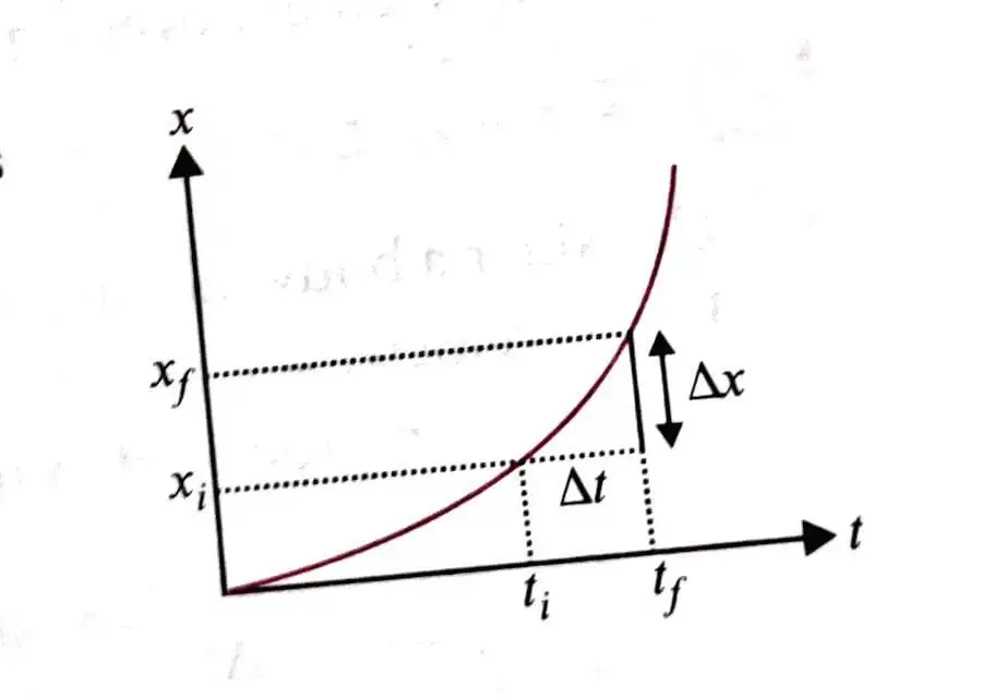
Instantaneous velocity — The rate of change of position with time at a particular instant.
The differential form gives velocity at time .
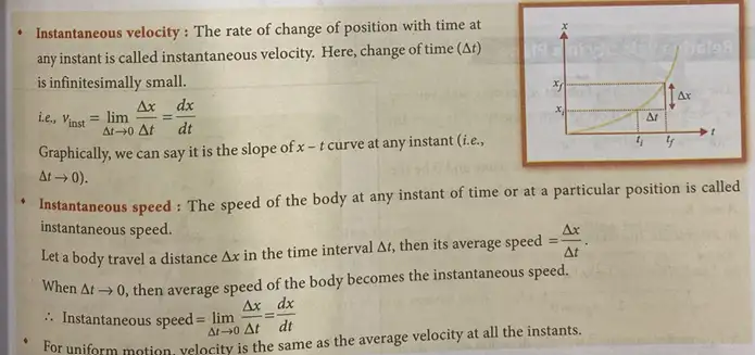
Instantaneous speed — The speed of an object at a particular instant or position.
The magnitude is used because speed has no direction.
- For uniform motion, velocity is constant and equals average velocity at every instant.
- On a position–time graph, secant slope gives average velocity; tangent slope gives instantaneous velocity.
Quick recap
- Rectilinear motion is motion along a straight line; kinematics describes motion without its causes.
- Distance follows the actual route, while displacement is the directed change from initial to final position.
- Distance is always at least as large as the magnitude of displacement.
- Average velocity is displacement divided by time; its graph interpretation is the secant slope.
- Average speed is total distance divided by total time and can differ from the magnitude of average velocity if direction reverses.
- Instantaneous velocity is ; instantaneous speed is its magnitude, and the position–time tangent slope gives instantaneous velocity.
Acceleration
Meaning and Direction of Acceleration
Acceleration — The rate of change of velocity with time; acceleration is a vector quantity.
Direction and Units
- Direction: Acceleration points in the direction of the change in velocity, not necessarily in the direction of velocity.
- Example: In circular motion, acceleration is directed towards the centre, while velocity is tangential.
- Units: SI unit is ; CGS unit is .
Net change in velocity divided by the elapsed time.
Acceleration at a particular instant; in straight-line motion, it is the second derivative of position with respect to time.
Types of Acceleration
| Type | Condition |
|---|---|
| Uniform acceleration | Both magnitude and direction remain constant. |
| Non-uniform acceleration | Magnitude, direction, or both change with time. |
Acceleration on Motion Graphs
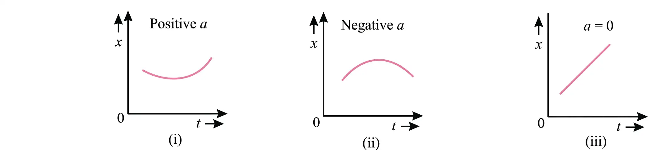
Position–Time Graph
- Positive acceleration: The position–time graph curves upward; its slope, representing velocity, increases.
- Negative acceleration: The position–time graph curves downward; its slope decreases.
- Zero acceleration: Velocity is constant, so position changes linearly with time and the graph is a straight line.
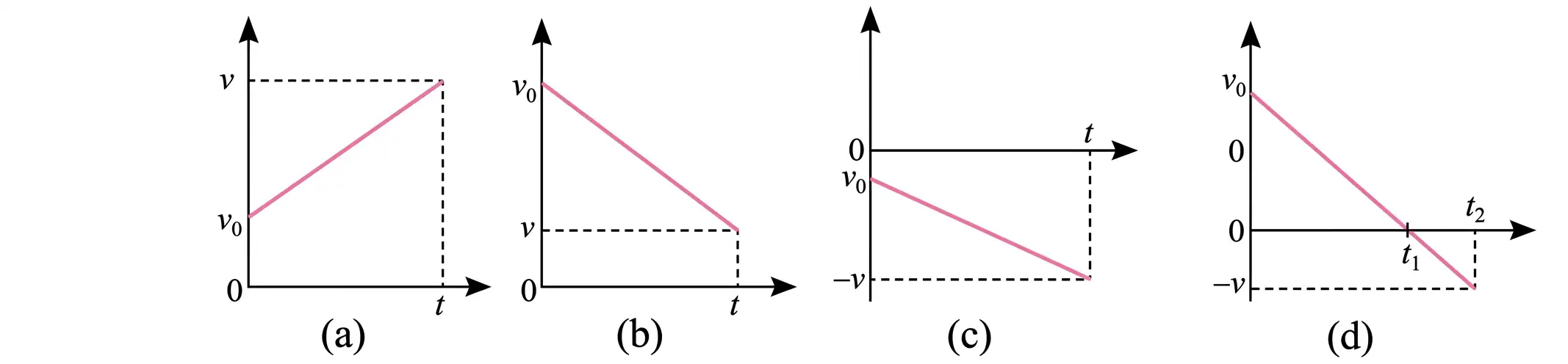
| Case | Velocity direction | Acceleration direction | Effect on speed |
|---|---|---|---|
| Motion in positive direction with positive acceleration | Positive | Positive | Speed increases. |
| Motion in positive direction with negative acceleration | Positive | Negative | Speed decreases. |
| Motion in negative direction with negative acceleration | Negative | Negative | Speed increases. |
| Negative acceleration with direction reversal | Positive before ; negative after | Negative throughout | Velocity reaches zero at , then motion reverses. |
Velocity–Time Graph
- Slope: The slope of a velocity–time graph gives acceleration; constant acceleration appears as a straight line.
- Area: The signed area under the velocity–time graph over a time interval gives displacement.
- Direction reversal: When velocity changes from positive to negative, the object moves in the positive -direction before crossing zero and in the negative -direction afterwards.
Displacement is the signed area under the graph between the chosen times.
Do not assume acceleration points in the direction of velocity: acceleration is directed along the change in velocity.
What does the area under a velocity–time graph represent?
Quick recap
- Acceleration is the vector rate of change of velocity; its SI and CGS units are and .
- Average acceleration is change in velocity divided by elapsed time; instantaneous acceleration is .
- Uniform acceleration has constant magnitude and direction; non-uniform acceleration changes in magnitude, direction, or both.
- For constant acceleration, velocity–time graphs are straight lines; their slope gives acceleration and signed area gives displacement.
- The sign of velocity gives direction of motion, while acceleration may point with or against that direction.
Kinematic Equations for Uniformly Accelerated Motion
Kinematic Equations from a Velocity–Time Graph
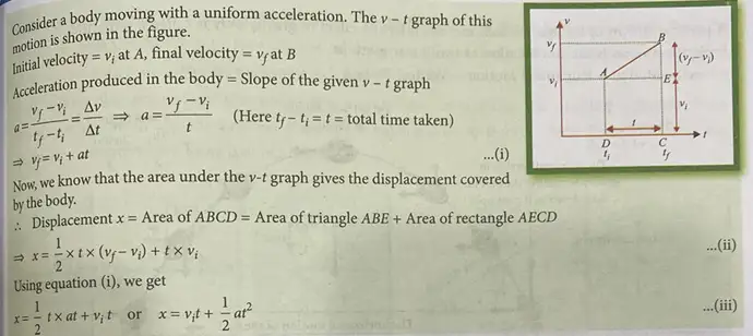
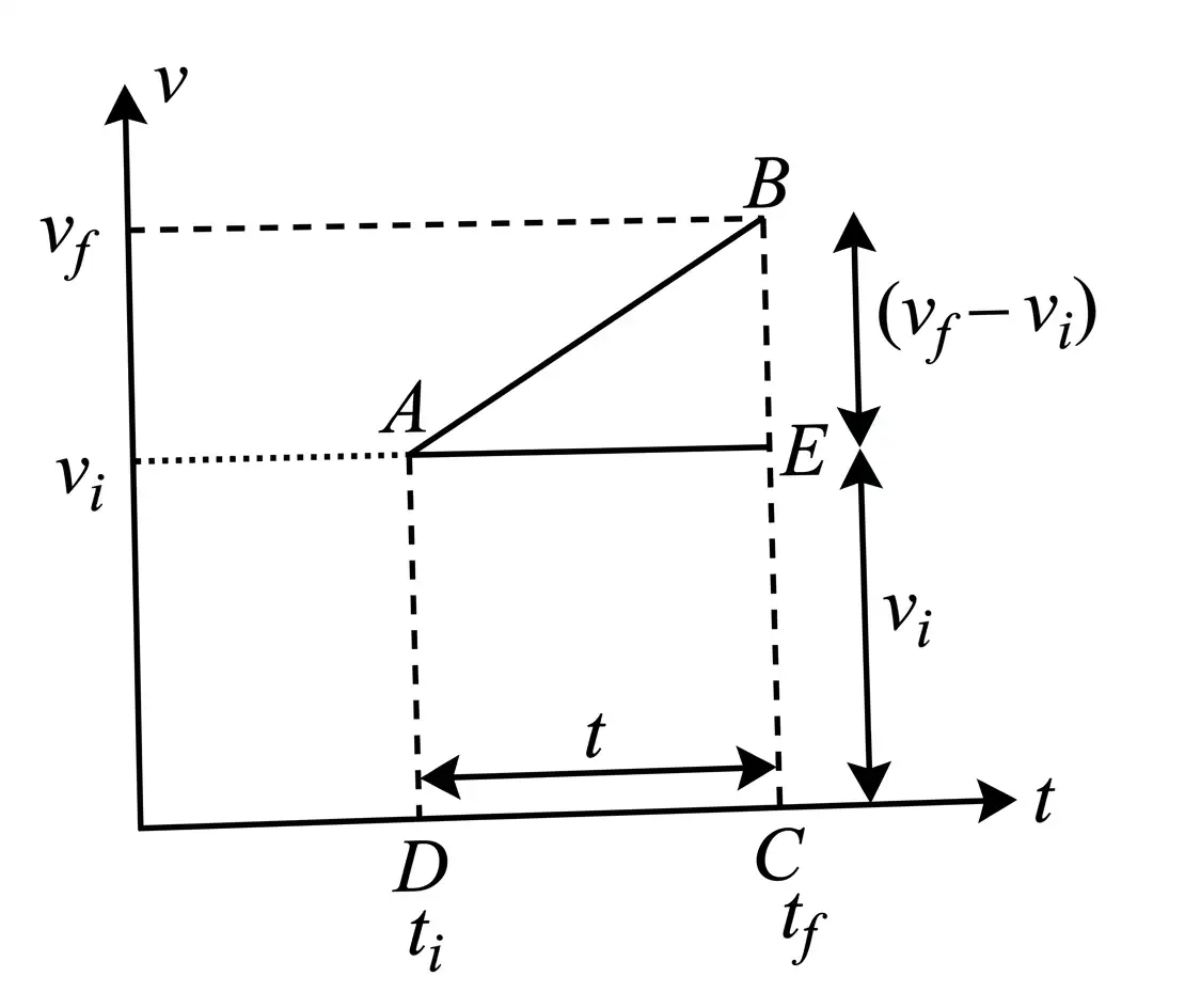
Acceleration equals change in velocity divided by elapsed time.
For initial velocity , final velocity , constant acceleration and elapsed time .
Displacement from the Graph
- Area: Displacement equals the rectangle plus the triangle under the velocity–time graph: .
- Substitution: Using gives the displacement equation for constant acceleration.
Displacement after time under constant acceleration.
Connects velocity and displacement without using time.
- Symbols: = initial velocity, = final velocity, = constant acceleration, = time, and = displacement.
- Condition: These equations apply to one-dimensional motion with constant acceleration.
Displacement in the nth Second
With time measured in seconds.
Motion Under Gravity
For initial upward speed , where is the magnitude of gravitational acceleration.
Vertical Upward Throw
- At maximum height: The instantaneous velocity is zero.
- Ascent and descent: For return to the launch level, time of ascent equals time of descent.
- Return: The body reaches the projection point with speed , directed downward.
For a body thrown vertically upward and returning to its launch level.
A body dropped from height reaches this speed, neglecting air resistance.
Relative Velocity
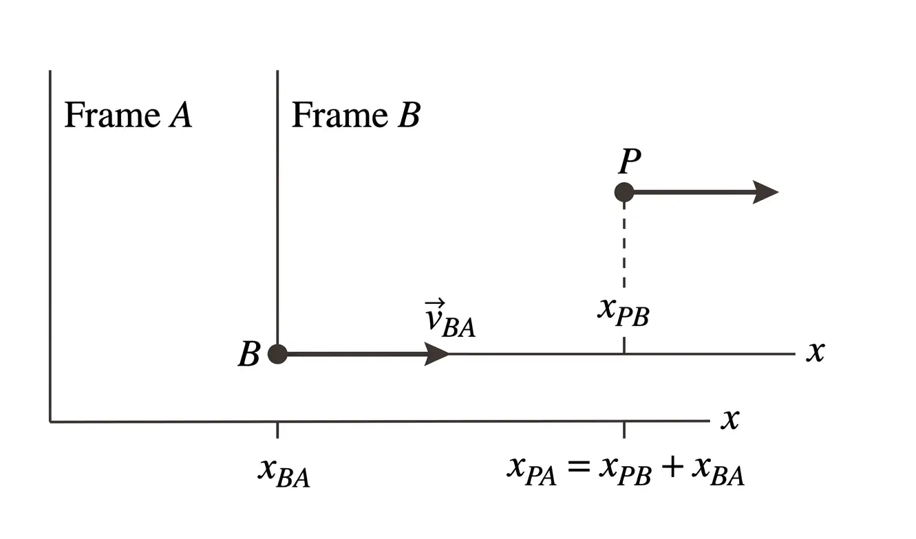
Position of object measured in frames and .
Differentiate the position relation with respect to time.
| Motion | Relative velocity of with respect to |
|---|---|
| Same direction | |
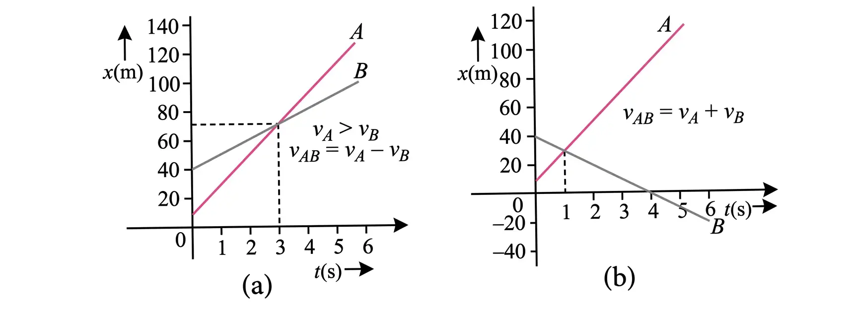
| Opposite directions | when and are positive speed magnitudes |
Reading Position–Time Graphs
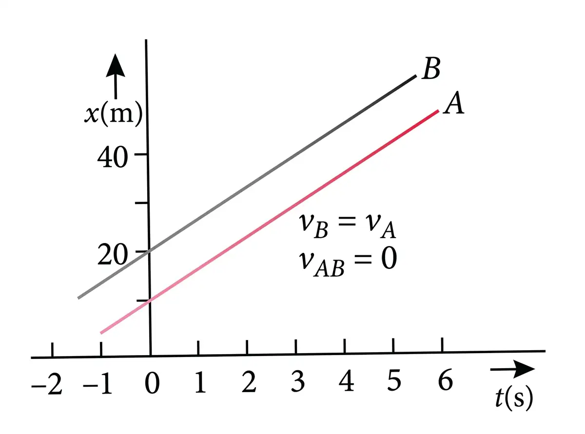
- Slope: The slope of a position–time graph gives velocity.
- Equal velocities: Parallel lines have equal slopes, so relative velocity is zero and separation stays constant.
- Meeting: The graphs intersect when the objects have the same position.
- Examples: The same-direction case meets at ; the opposite-direction case meets at .
State the three kinematic equations for constant acceleration.
What is the total time of flight for an upward throw that returns to its launch level?
How do you find the relative velocity of with respect to ?
Quick recap
- A velocity–time graph’s slope gives acceleration; its area gives displacement.
- Acceleration is , and the constant-acceleration equations connect velocity, time and displacement.
- Displacement during the nth second is .
- For free fall, use the kinematic equations with and choose signs consistently.
- For an upward throw, maximum height is and total flight time is .
- Relative velocity is found by subtracting signed velocities; parallel position–time lines mean zero relative velocity.
NEET Physics — ALL CHAPTERS
1
Basic Mathematics
2
Units and Measurement
3
Motion in a Straight Line
4
Motion in a Plane
5
Laws of Motion
6
Work, Energy and Power
7
System of Particles and Rotational Motion
8
Gravitation
9
Mechanical Properties of Solids
10
Mechanical Properties of Fluids
11
Thermal Properties of Matter
12
Thermodynamics
13
Kinetic Theory
14
Oscillations
15
Waves
16
Electric Charges and Fields
17
Electrostatic Potential and Capacitance
18
Current Electricity
19
Moving Charges and Magnetism
20
Magnetism and Matter
21
Electromagnetic Induction
22
Alternating Current
23
Electromagnetic Waves
24
Ray Optics and Optical Instruments
25
Wave Optics
26
Dual Nature of Radiation and Matter
27
Atoms
28
Nuclei
29
Semiconductor Electronics: Materials, Devices and Simple Circuits