NEET UG . NEET Physics . Physics . Motion in a Plane
Chapter 4: Motion in a Plane
Ch 4
NEET Physics
NEET UG
Scalars and Vectors
Scalar and Vector Quantities
Why vectors are needed
- Motion in a plane: Describing motion in more than one dimension requires vectors to represent direction as well as magnitude.
- Applications: Velocity and acceleration in a plane are described using vectors.
Scalar — A scalar is a physical quantity specified completely by its magnitude and unit.
Scalar operations and examples
- Direction: Scalars have magnitude but no direction.
- Operations: Scalars are combined using ordinary algebra and can be added, subtracted, multiplied or divided.
- Units: Addition and subtraction require quantities with the same units; multiplication and division can combine different units.
- Examples: Distance, speed and temperature are scalars.
| Quantity | Example |
|---|---|
| Perimeter of a rectangle | |
| Density |
Vector — A vector is a physical quantity with both magnitude and direction that obeys the triangle law of addition.
Representation and notation
- Diagram: A vector is drawn as a line with an arrowhead; its length represents magnitude and its arrowhead shows direction.
- Endpoints: The starting end is the tail or initial point; the arrowhead end is the head or terminal point.
- Notation: A vector may be written with an arrow, such as , or in bold type in books.
- Modulus: The magnitude of is its modulus, written as or .
- Example: Velocity and acceleration are vector quantities.
Position and Displacement Vectors
Position vector — A position vector specifies an object's position relative to the origin of a coordinate system.
- Information given: It gives both the straight-line distance from the origin and the direction from the origin.
- Notation: For an object at , its position vector is .
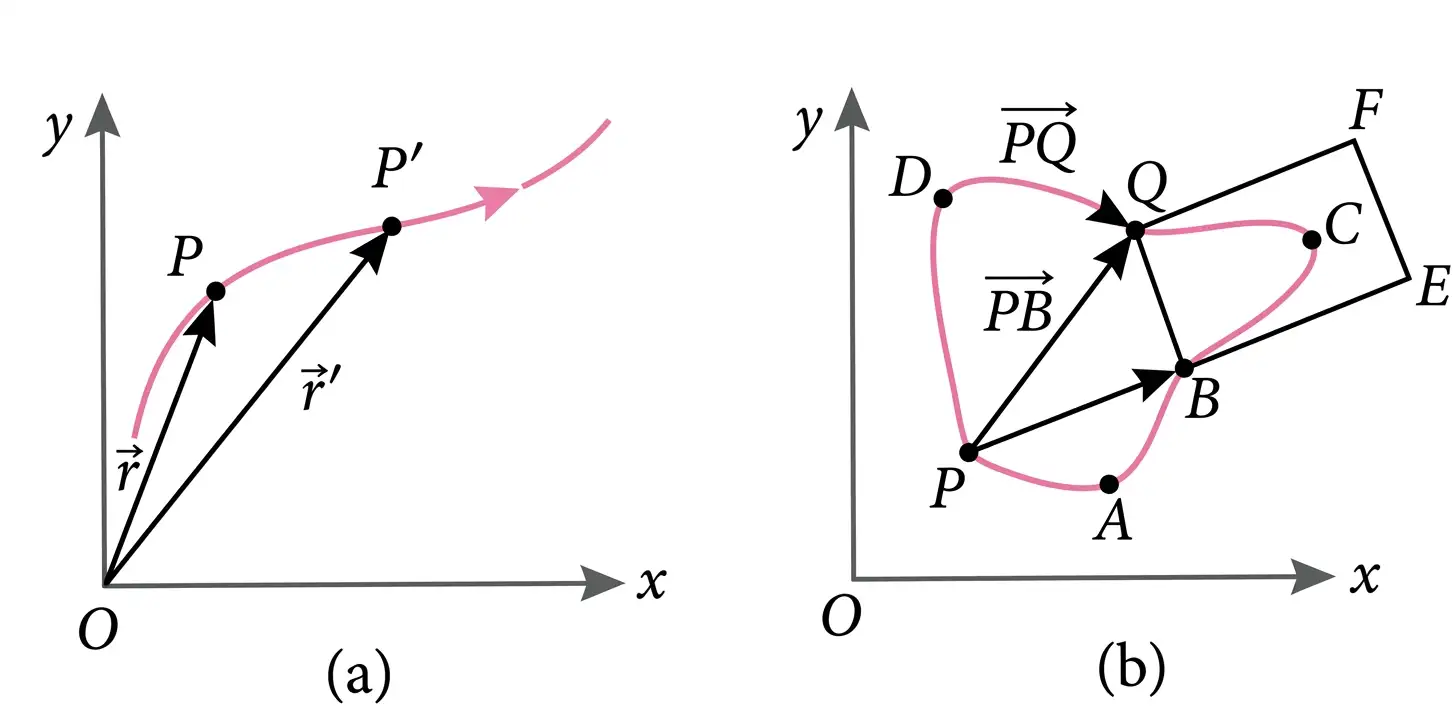
Displacement vector — A displacement vector describes the change in an object's position, including how far and in which direction it moved.
- Straight-line change: Displacement is the straight line from the initial position to the final position; it does not depend on the route taken.
- Relation: If initial and final position vectors are and , then .
- Magnitude: The magnitude of displacement is less than or equal to the path length between the two positions.
- Example: Different routes from to have the same displacement vector .
Equality and Scalar Multiplication of Vectors
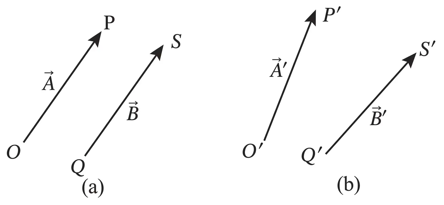
Equal vectors — Two vectors are equal if and only if they have the same magnitude and the same direction.
- Location: Equal vectors need not start at the same point; translating a vector without changing its magnitude or direction preserves it.
- Unequal vectors: Vectors of equal length are not equal if their directions differ.
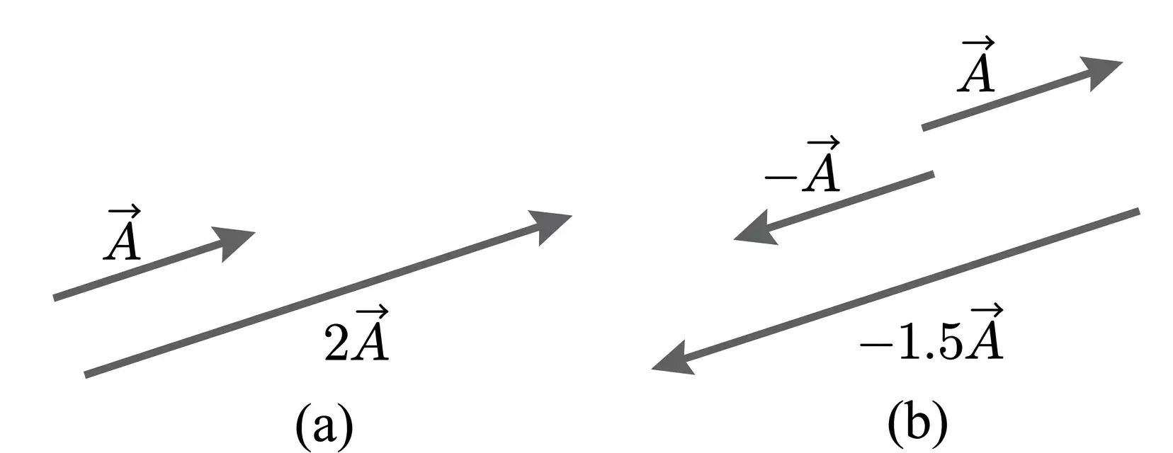
Multiplying a vector by a scalar
- Magnitude: Multiplying by a scalar changes its magnitude to .
- Positive scalar: If , the vector's direction remains unchanged.
- Negative scalar: If , the vector's direction reverses.
What conditions must two vectors satisfy to be equal?
How does displacement differ from path length?
Quick recap
- Scalars have magnitude only; vectors have magnitude and direction.
- Scalar addition and subtraction require matching units; multiplication and division may involve different units.
- A vector's arrow length shows magnitude and its arrowhead shows direction.
- A position vector locates an object relative to the origin.
- Displacement is the straight-line change in position, regardless of the route taken.
- Equal vectors have the same magnitude and direction, even if they start at different points.
- Multiplying a vector by a positive scalar preserves its direction; a negative scalar reverses it.
Multiplication of Vectors by Real Number
Scalar Multiplication of a Vector
Use this relation to calculate the magnitude after scalar multiplication.
Examples
- Multiply by : has magnitude and points in the same direction as .
- Multiply by : has magnitude and points opposite to .
- Multiply by : has magnitude and points opposite to .
Do not use for the magnitude when is negative; magnitude is non-negative, so use .
Quick recap
- Scalar multiplication of a vector by a real number gives another vector.
- The product's magnitude is .
- A positive scalar preserves the vector's direction.
- A negative scalar reverses the vector's direction.
- Multiplication by zero gives the zero vector.
- points along ; and point opposite to it.
Addition and Subtraction of Vectors – Graphical Method
Vector Addition
Head-to-tail rule — Arrange vectors so the head of each vector meets the tail of the next; the resultant runs from the first tail to the final head.
Properties of vector addition
- Commutative: The order of adding vectors does not change the resultant: .
- Associative: The grouping of vectors does not change the resultant: .
- Distributive: Scalar multiplication distributes over vector addition: .
Triangle Law of Vector Addition
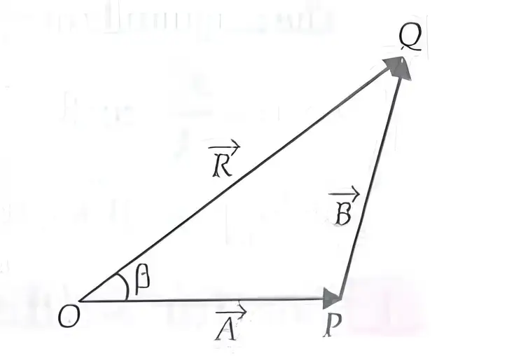
Triangle law — If two vectors are represented by two sides of a triangle in the same order, their sum is represented by the third side taken in the opposite order.
- Resultant: For vectors and , the resultant is .
- Construction: Draw from the head of ; draw from the tail of to the head of .
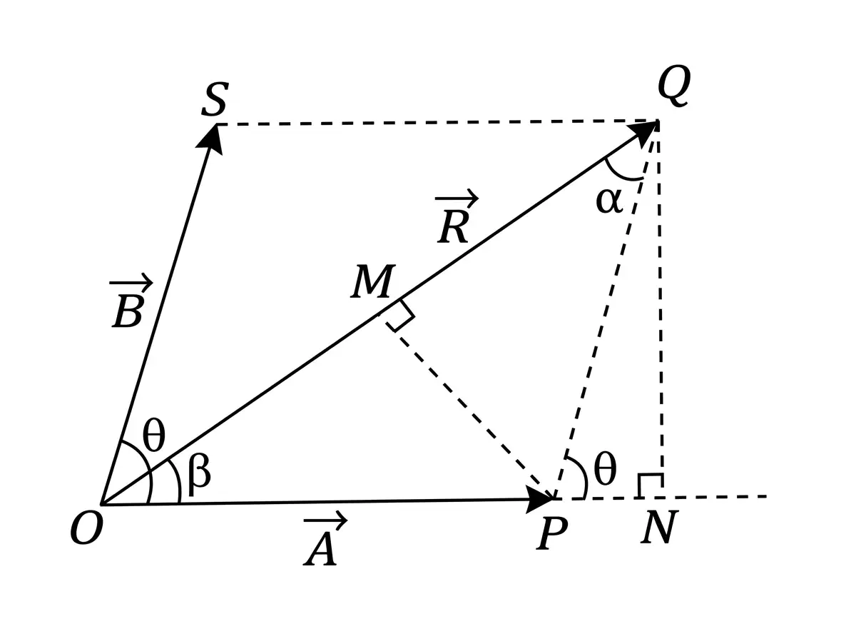
Parallelogram Law of Vector Addition
Parallelogram law — If two vectors from the same point are represented by adjacent sides of a parallelogram, their resultant is the diagonal from that point.
- Angle: Let be the angle between and ; let be the angle between and the resultant.
- Magnitude and direction: The formulas give the resultant’s magnitude and its direction relative to .
Use when the angle between the two vectors is .
Here, is measured from toward .
Polygon Law of Vector Addition
Polygon law — If several vectors form successive sides of an open polygon in the same order, their resultant is the closing side taken in the opposite order.
Special Cases of Vector Addition
| Arrangement | Resultant magnitude | Direction |
|---|---|---|
| Same direction | Along both vectors; from | |
| Opposite directions | Along the larger vector; zero if | |
| Mutually perpendicular | from toward |
Vector Subtraction
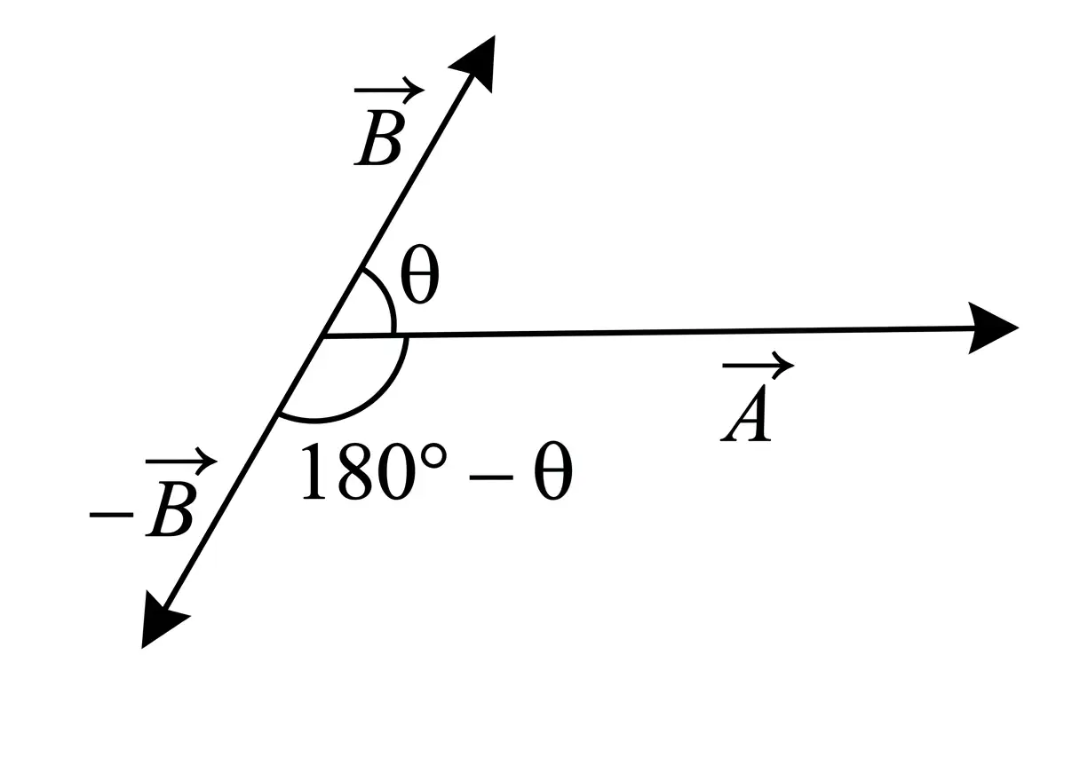
Vector subtraction — Subtracting from means adding the negative of to .
- Negative vector: has the same magnitude as but points in the opposite direction.
- Supplementary angle: If the angle between and is , the angle between and is .
For angle between and .
Properties of vector subtraction
- Not commutative: In general, .
- Not associative: In general, .
State the triangle law of vector addition.
How is vector subtraction defined, and what is the magnitude of the difference?
Quick recap
- Use the head-to-tail construction to obtain a vector sum.
- Vector addition is commutative, associative and distributive over scalar multiplication.
- Triangle, parallelogram and polygon laws are graphical constructions for vector addition.
- For two vectors at angle , .
- Subtracting a vector means adding its opposite; the difference magnitude uses the minus sign before .
- Vector subtraction is generally neither commutative nor associative.
Resolution of Vectors
Resolution and Components
Resolution of a vector — The process of splitting a vector into two or more vectors is called resolution of a vector.
- Component vectors are the vectors into which the original vector is resolved.
- Rectangular components are components along mutually perpendicular directions.
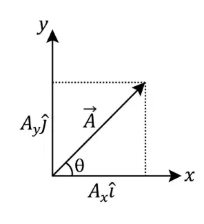
Rectangular Components in a Plane
- Setup: If vector makes an angle with the positive -axis, its rectangular components lie along the - and -axes.
- Components: and .
- Magnitude and direction: and .
The vector is the sum of its perpendicular components.
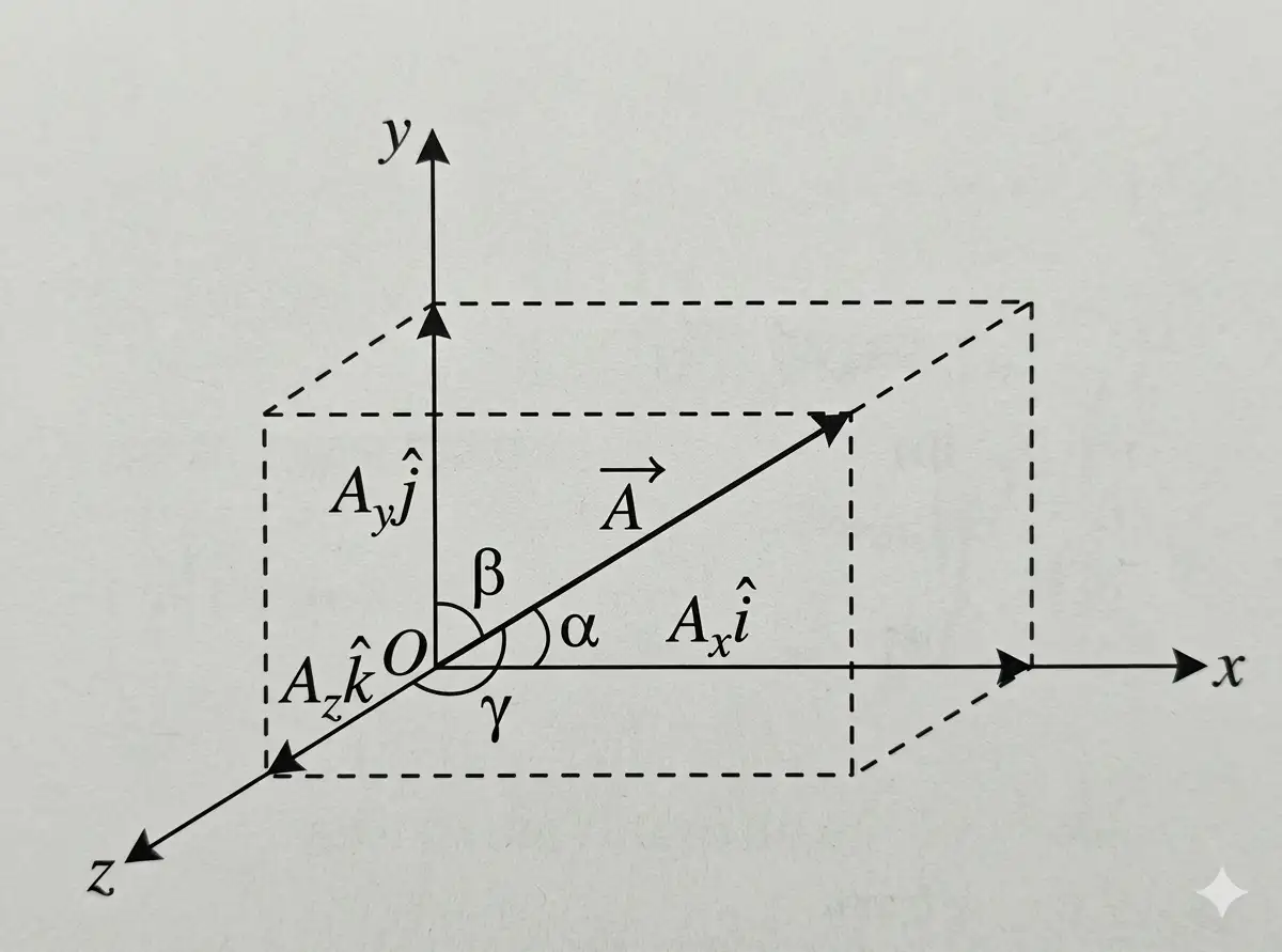
Rectangular Components in Space
- Setup: Let , and be the angles made by vector with the -, - and -axes, respectively.
- Components: , and .
- Magnitude: The vector’s magnitude is .
- Direction cosines: , and ; these are the direction cosines of .
The vector is the sum of its three mutually perpendicular components.
The squares of the three direction cosines add to unity.
Quick recap
- Resolution splits a vector into component vectors.
- Rectangular components act along mutually perpendicular axes.
- In a plane, and .
- In space, the components are , and .
- The 3D magnitude is .
- The direction cosines satisfy .
Vector Addition -Analytical Method
Adding Vectors by Components
Use these relations to add two vectors in the - plane.
Add the components along each axis separately.
Addition in Three Dimensions
The resultant components are the sums of the corresponding components.
Add each pair of components along the same axis.
Adding and Subtracting Any Number of Vectors
For vectors in three dimensions, add all components along each axis.
Subtract corresponding components.
Quick recap
- Represent each vector by its components along the coordinate axes.
- Add corresponding components to find the resultant.
- In two dimensions, use the - and -components.
- In three dimensions, add the -, - and -components.
- The same component-wise method works for any number of vectors and for subtraction.
Motion in a Plane
Position and Displacement Vectors
Here, and are unit vectors along the - and -axes.
Displacement vector — Displacement is the change in position, directed from the initial point to the final point.
For motion from to , the changes in coordinates are and .
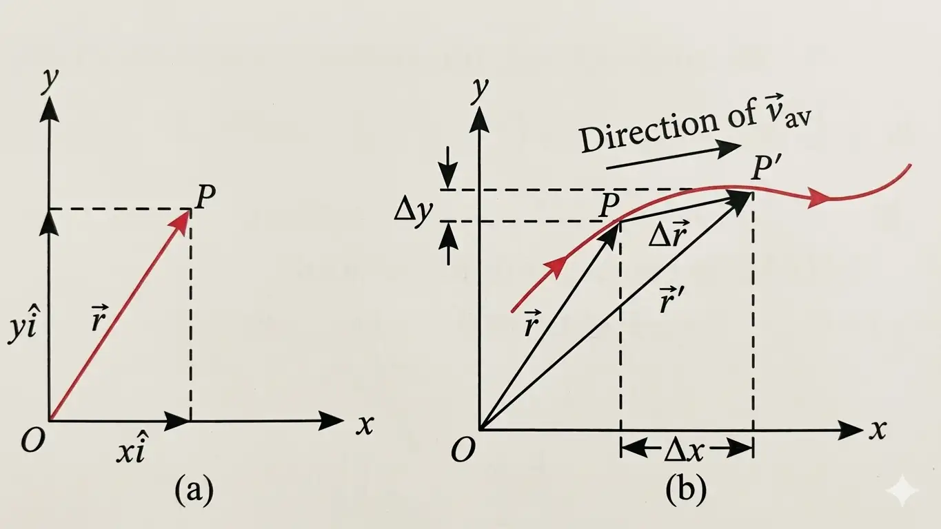
Velocity
The component form follows by dividing each displacement component by .
Instantaneous velocity — Instantaneous velocity is the limiting value of average velocity as the time interval approaches zero.
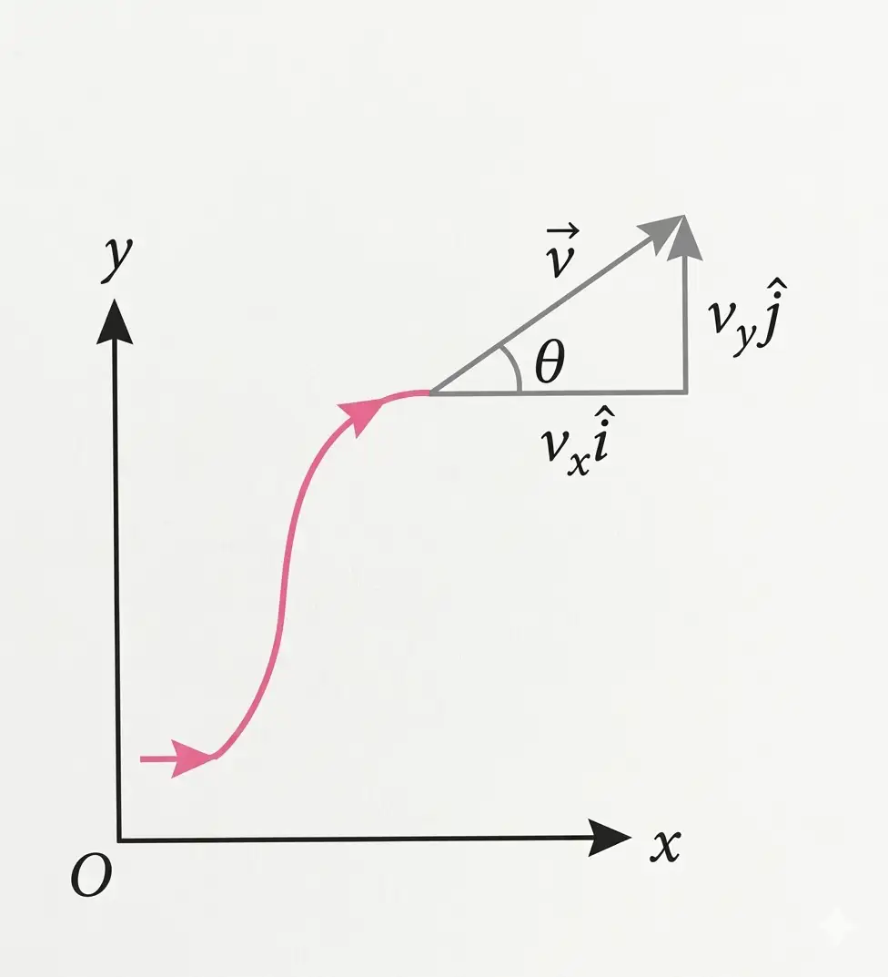
The vector derivative gives the instantaneous velocity and its components.
The angle is measured from the positive -axis.
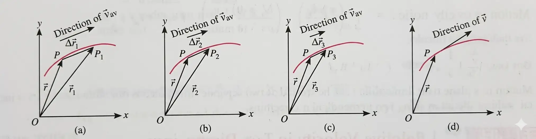
Acceleration
The components are and .
Instantaneous acceleration — Instantaneous acceleration is the limiting value of average acceleration as the time interval approaches zero.
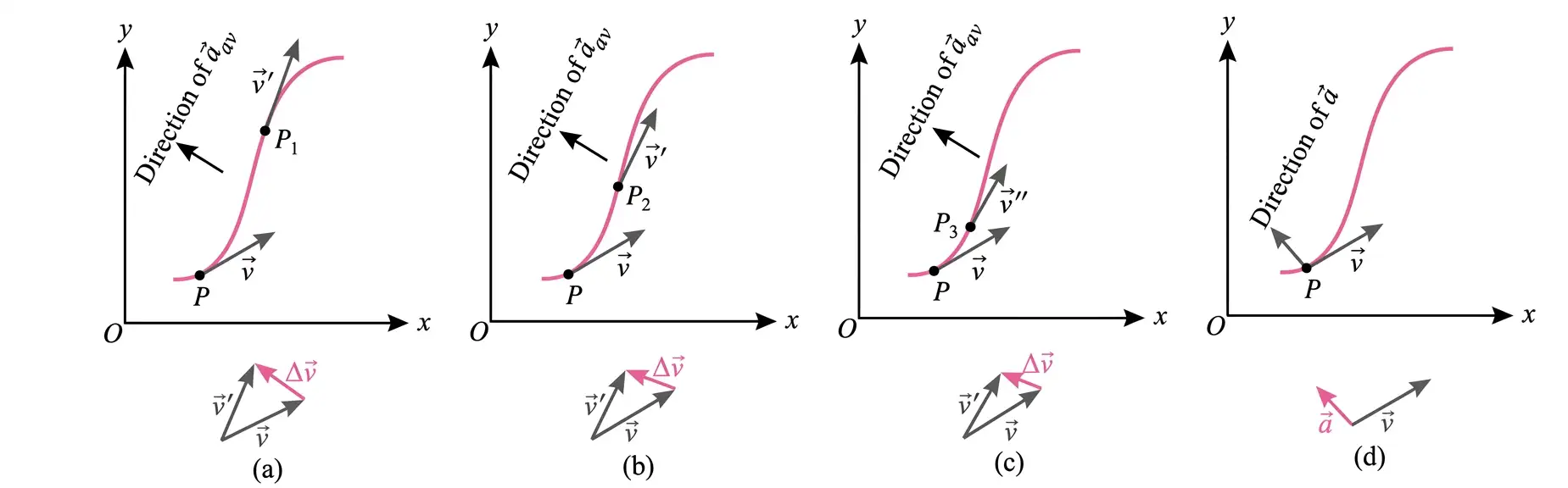
Quick recap
- A position vector gives a particle’s location: .
- Displacement is the final position minus the initial position: .
- Average velocity is displacement per time interval; instantaneous velocity is .
- Instantaneous velocity is tangent to the path and points in the direction of motion.
- The velocity magnitude is , with .
- Average acceleration is ; instantaneous acceleration is .
Motion in a Plane with Constant Acceleration
Constant Acceleration in Two Dimensions
Constant acceleration — Acceleration is constant when the velocity changes by equal vector amounts in equal time intervals.
Motion equations
- Velocity: For initial velocity and constant acceleration , velocity after time is given by .
- Average velocity: Over the interval from to , .
- Displacement: The position after time is .
- Components: Resolve the motion along perpendicular axes and apply the one-dimensional equations separately.
Use each equation independently along its axis.
Two-dimensional motion is treated as simultaneous one-dimensional motions along perpendicular directions.
Relative Velocity in Two Dimensions
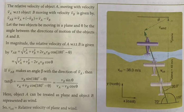
Relative velocity — The velocity of an object measured with respect to a moving reference object is its relative velocity.
Reference frames and vector relation
- Actual velocity: Velocity of the particle measured from the ground frame.
- Relative velocity: Velocity of the particle measured from the moving frame.
- Reference velocity: Velocity of the moving frame relative to the ground.
- Vector addition: Position vectors add as ; differentiating with respect to time gives the velocity relation.
Actual velocity equals relative velocity plus reference velocity; rearrange to find relative velocity.
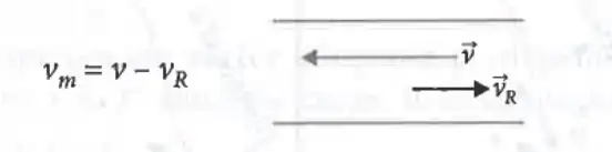
Swimming in a River
Swimming relative to the water and ground
- Swimmer's velocity: Let be the swimmer's velocity relative to still water and the river's velocity relative to the ground.
- Ground velocity: The swimmer's velocity relative to the ground is .
- Downstream: If the swimmer moves with the current, the speeds add: .
- Upstream: If the swimmer moves against the current, the ground speed is ; upstream progress requires .
- Across the river: When the two velocities are not collinear, add them as vectors and resolve into components.
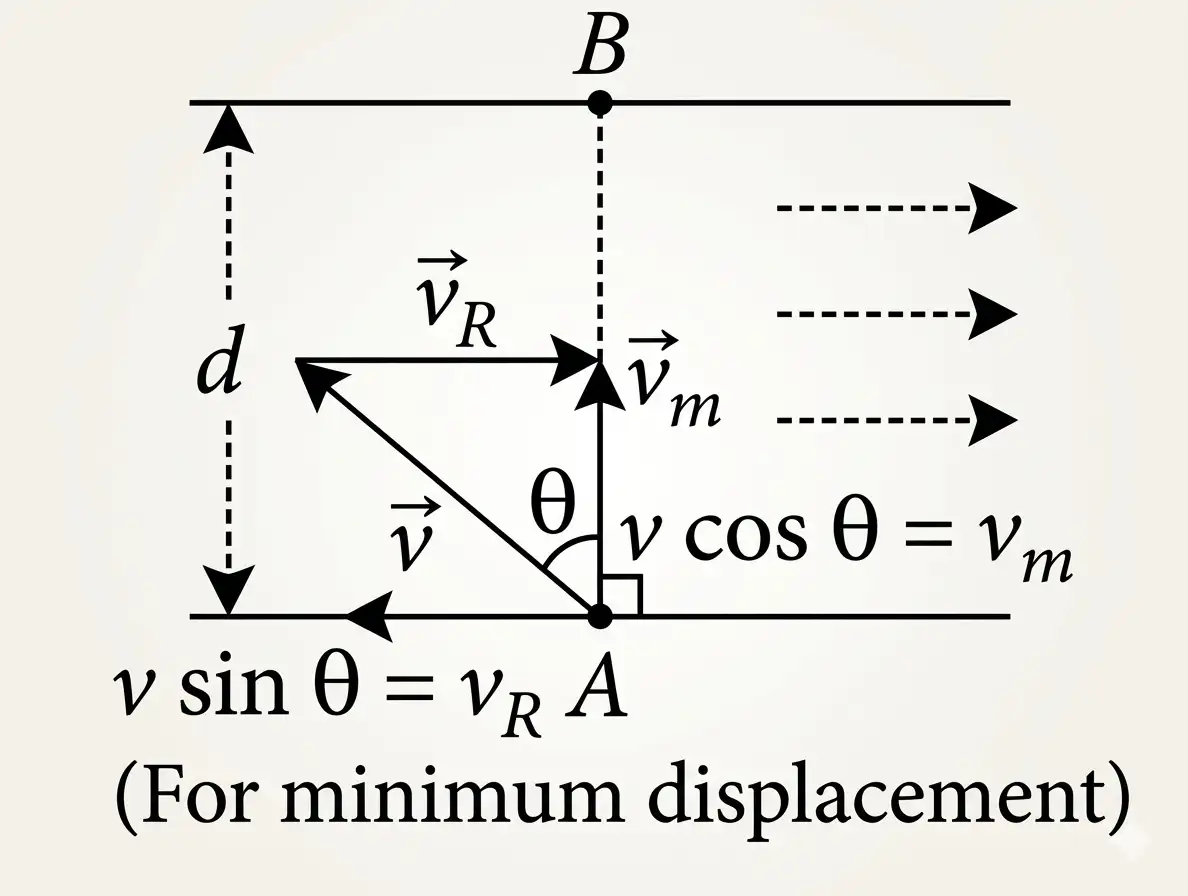
Shortest Path and Minimum Time
| Point | Shortest path | Minimum time |
|---|---|---|
| Direction of swimmer | Aim upstream so the resultant velocity points directly across the river. | Swim perpendicular to the current. |
| Crossing time | , provided . | . |
| Drift | No downstream drift for the direct path. | The current carries the swimmer downstream by . |
Shortest-path condition
- Cancellation: For a straight path directly across, the swimmer's upstream component cancels the river current: .
- Angle: Thus , where is measured from the direction perpendicular to the river flow.
- Across-river speed: The resultant component across the river is .
- Time: For river width , the crossing time is .
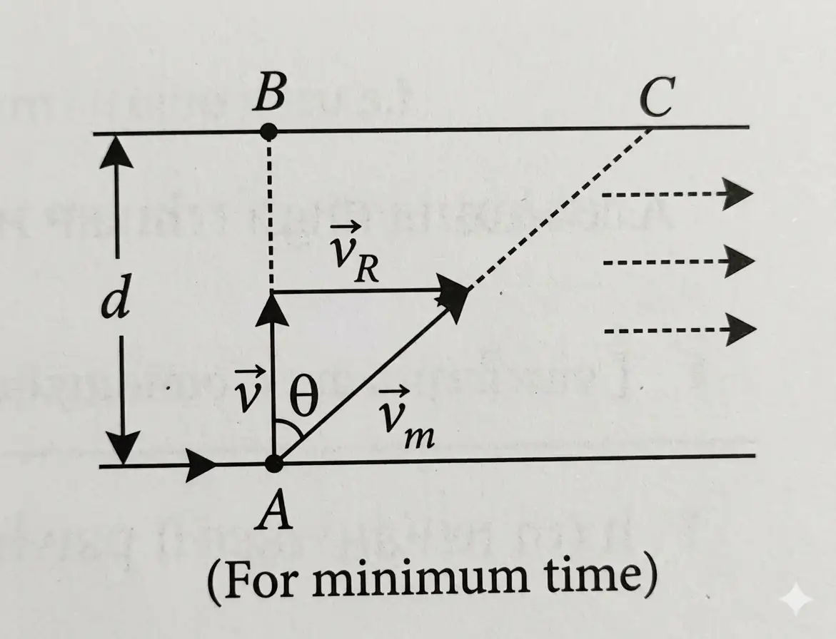
Minimum-time condition
- Direction: Swim perpendicular to the current so the full swimmer speed contributes to crossing.
- Crossing time: For river width , .
- Drift: During this time the river carries the swimmer downstream: .
- Key distinction: Minimum time does not give the shortest path because the swimmer drifts downstream.
Rain Problem
Apparent velocity of rain — The rain's velocity relative to a moving person determines the direction from which the rain appears to fall.
Rain relative to a moving person
- Ground-frame rain velocity: If rain has components horizontally and vertically downward, then .
- Rain speed: Its magnitude is .
- Ground-frame angle: The angle from the vertical satisfies .
- Person's velocity: For a person moving horizontally at speed , .
- Relative rain velocity: Subtract the person's ground velocity: .
- Umbrella direction: The umbrella should point against the apparent rain velocity; the apparent angle from the vertical obeys .
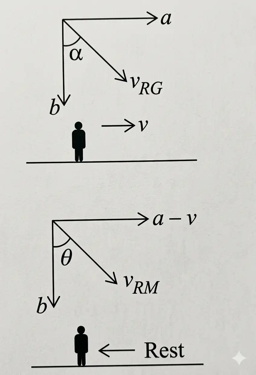
Do not subtract speeds without considering directions. Relative velocity is a vector difference: .
How should a swimmer aim to cross a river along the shortest path?
What is the minimum crossing time and downstream drift?
Quick recap
- Constant-acceleration motion in two dimensions is solved independently along perpendicular axes.
- Velocity changes as ; position follows .
- Actual velocity equals relative velocity plus reference velocity.
- Downstream and upstream speeds combine according to the direction of the river current.
- Shortest-path crossing cancels current drift; minimum-time crossing swims perpendicular to the current and results in drift.
- Rain's apparent direction is found by subtracting the observer's velocity from the rain's ground velocity.
Projectile Motion
Projectile motion — The motion of a body projected at an angle to the horizontal under gravity alone is called projectile motion.
Model and assumptions
- Projectile: The body in motion is called a projectile.
- Assumptions: Neglect air resistance and the Earth's curvature and rotation; acceleration is due to gravity alone.
- Axes: Take the horizontal as the -axis and the vertical as the -axis; motion lies in this plane.
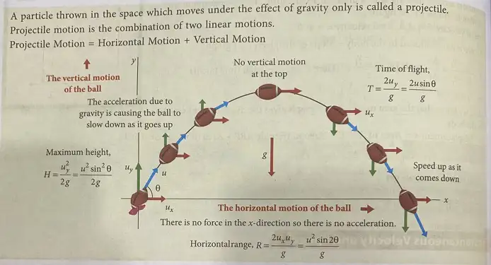
Motion along the horizontal and vertical axes
Resolve the initial velocity
- Initial velocity: For launch speed at angle above the horizontal, and .
- Horizontal motion: Acceleration is zero, so horizontal velocity remains constant.
- Vertical motion: Taking upward as positive, acceleration is .
Treat the horizontal and vertical motions independently to solve projectile-motion problems.
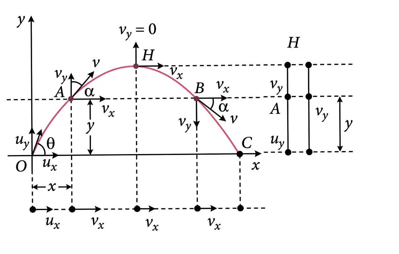
Trajectory of a projectile
Eliminate time using . The trajectory is a downward-opening parabola.
Velocity at any time
- Speed: Combine the perpendicular components: .
- Direction: If the velocity makes angle with the horizontal, then .
Time of flight
Time of flight — The time for which a projectile remains in the air, from projection to landing at the same vertical level.
Set the vertical displacement to zero at landing, excluding the launch-time solution .
- Symmetry: With no air resistance and equal launch and landing heights, time of ascent equals time of descent; each is .
Maximum height
Maximum height — The greatest vertical displacement reached by the projectile above its point of projection.
At the highest point, vertical velocity is zero while horizontal velocity remains .
Horizontal range
Horizontal range — The horizontal distance travelled by a projectile during its time of flight.
For launch and landing at the same level, range equals horizontal speed multiplied by time of flight.
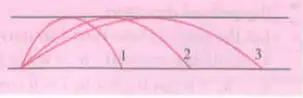
Comparing projectiles with different launch angles
Same vertical component
- Equal vertical components: If projectiles have the same , they reach the same maximum height and have the same time of flight.
- Range comparison: Since , range increases with when is fixed.
- Ordering: If , then ; with equal , the launch speeds satisfy .
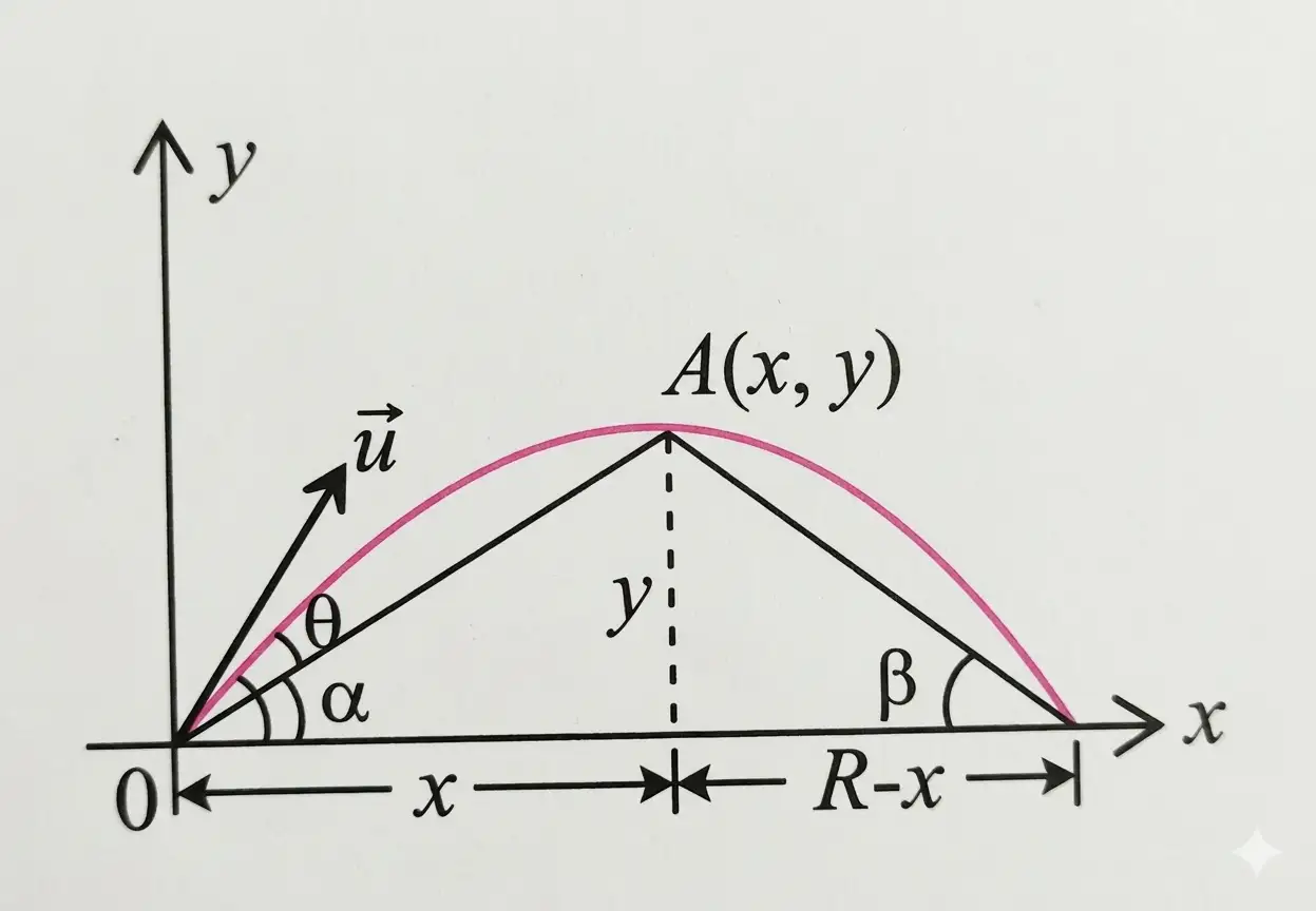
Launch angle from a point on the trajectory
- Geometry: For a point on a trajectory of total range , let and .
- Relation: The launch angle satisfies .
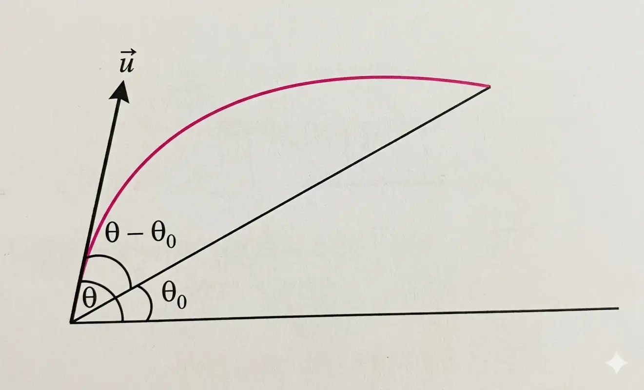
Projectile motion on an inclined plane
- Setup: Launch with speed at angle to the horizontal; the plane rises at angle to the horizontal.
- Range: Here is measured along the inclined plane, not horizontally.
These formulas apply when the projectile lands on the inclined plane; is measured from the horizontal.
For fixed launch speed, the maximum range occurs at the launch angle shown, measured from the horizontal.
Why is the trajectory of a projectile parabolic?
State the time of flight, maximum height, and range for a projectile landing at its launch level.
Quick recap
- Resolve launch velocity into and .
- Horizontal motion has constant velocity; vertical acceleration is .
- The trajectory is a downward-opening parabola.
- For equal launch and landing levels, .
- Maximum height is ; horizontal range is .
- On an incline, is measured from the horizontal and the range is measured along the plane.
Uniform Circular Motion
Angular Position and Displacement
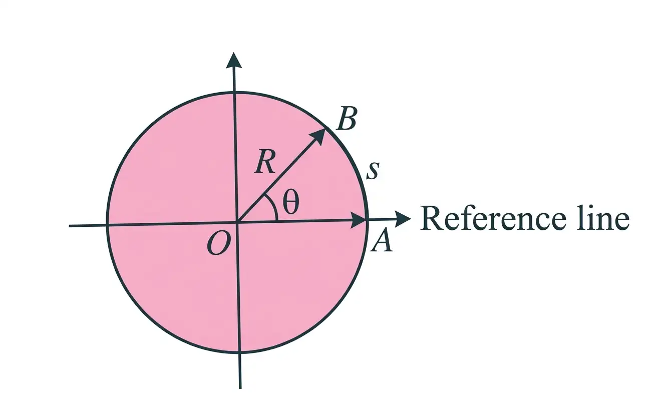
Angular position — The angle made by a particle’s radius vector with a chosen reference line.
Angular displacement — The angle through which the radius vector turns during a time interval; it is measured in radians.
For a circle of radius , arc length and angular displacement are related by this equation.
Angular Velocity
Average angular velocity — Total angular displacement divided by the time interval over which it occurs.
For angular positions and at times and :
Instantaneous angular velocity — The rate at which the radius vector rotates about the centre at a particular instant.
It is the limiting average angular velocity as the time interval approaches zero.
If rotations are completed in time , angular velocity is in radians per second. For period and frequency , use the equivalent relations below.
Uniform Circular Motion and Linear Velocity
Uniform circular motion — Motion along a circular path at constant speed.
Key features
- Speed: Remains constant, but the direction of linear velocity changes continuously.
- Angular velocity: Remains constant in uniform circular motion.
- Acceleration: Its magnitude is constant, but its direction continually changes.
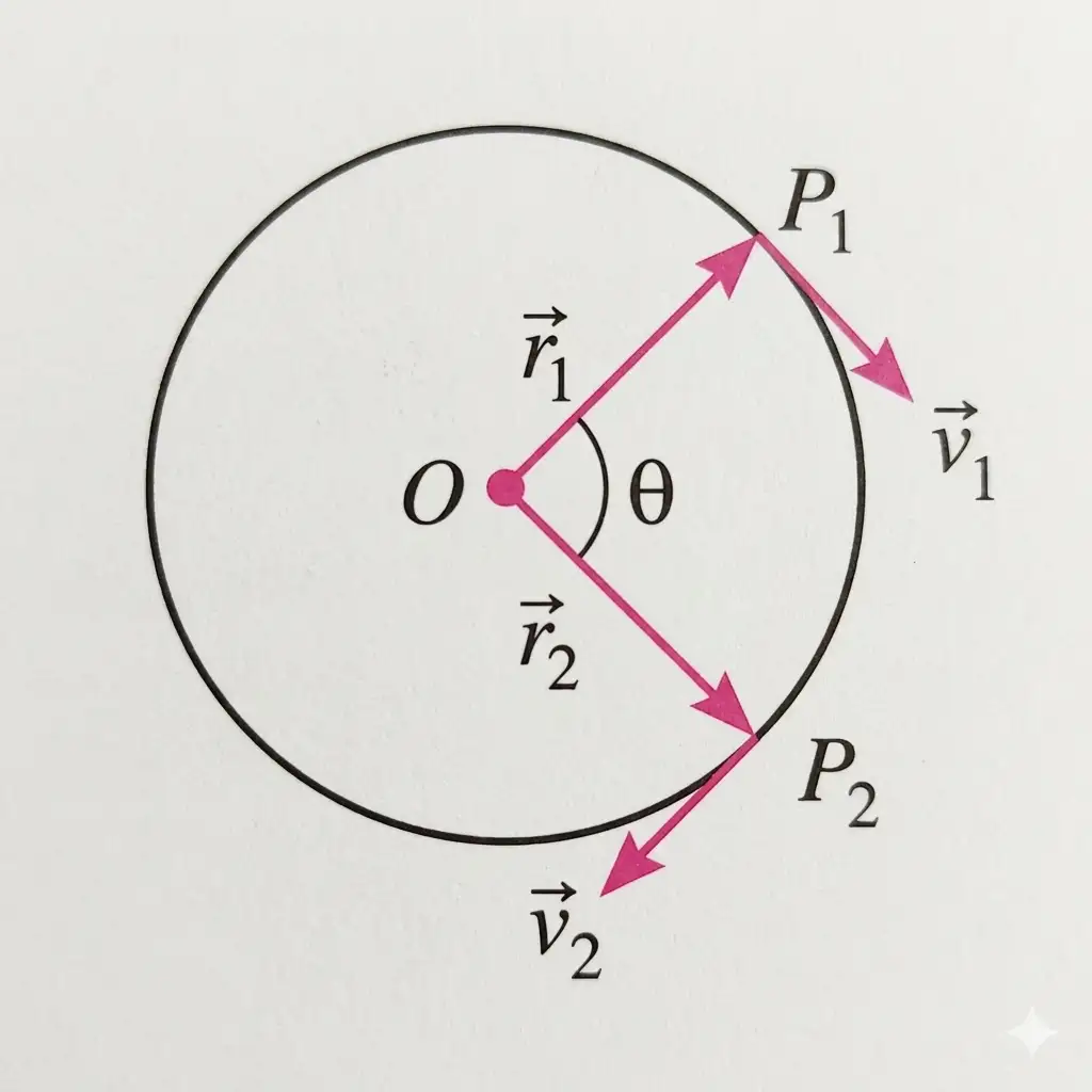
Relation between angular and linear speed
- In time , the particle covers arc length .
- At constant linear speed, the same arc length is .
- Equating the two: , so .
For a circle of radius , period is the time for one revolution; frequency is the number of revolutions per unit time.
Acceleration points toward the centre of the circular path.
Velocity relation
- Direction: Linear velocity is tangent to the circular path and perpendicular to the radius.
- Vector relation: The velocity vector is given by the cross product of angular velocity and position vector: .
Centripetal Force and Work
Centripetal force — The net inward force that provides the centripetal acceleration needed for circular motion.
For a particle of mass , the net tangential force is zero in uniform circular motion.
Work and power
- Direction: Centripetal force is always perpendicular to the instantaneous velocity; its direction changes as the particle moves.
- Work: It does no work, so it cannot change the particle’s kinetic energy.
- Power: The instantaneous power of centripetal force is zero: .
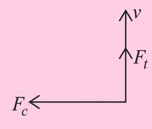
Constant speed does not mean constant velocity: the direction changes continuously. Centripetal force changes velocity’s direction, not its magnitude.
How are linear speed and angular speed related in uniform circular motion?
Why does centripetal force do no work in uniform circular motion?
Quick recap
- Angular displacement and arc length are related by .
- Angular velocity is ; for period and frequency , .
- In uniform circular motion, speed is constant while velocity direction changes continuously.
- Linear speed and angular speed are related by .
- Centripetal acceleration is and points inward.
- Centripetal force is perpendicular to velocity, does no work, and has zero power.
NEET Physics — ALL CHAPTERS
1
Basic Mathematics
2
Units and Measurement
3
Motion in a Straight Line
4
Motion in a Plane
5
Laws of Motion
6
Work, Energy and Power
7
System of Particles and Rotational Motion
8
Gravitation
9
Mechanical Properties of Solids
10
Mechanical Properties of Fluids
11
Thermal Properties of Matter
12
Thermodynamics
13
Kinetic Theory
14
Oscillations
15
Waves
16
Electric Charges and Fields
17
Electrostatic Potential and Capacitance
18
Current Electricity
19
Moving Charges and Magnetism
20
Magnetism and Matter
21
Electromagnetic Induction
22
Alternating Current
23
Electromagnetic Waves
24
Ray Optics and Optical Instruments
25
Wave Optics
26
Dual Nature of Radiation and Matter
27
Atoms
28
Nuclei
29
Semiconductor Electronics: Materials, Devices and Simple Circuits