NEET UG . NEET Physics . Physics . Electric Charges and Fields
Chapter 16: Electric Charges and Fields
Ch 16
NEET Physics
NEET UG
Electric Charge
Static Electricity and Electrostatics
Electrostatics — The study of forces, fields and potentials arising from static electric charges.
- Electric shocks can occur when electric charges discharge through the body, such as after sliding across a car seat.
- Static electricity is generated when electric charges discharge through the body.
Electric Charge
- Charging by electron transfer: a neutral body becomes charged when it gains or loses electrons.
- Electron loss leaves an object positively charged; electron gain makes it negatively charged.
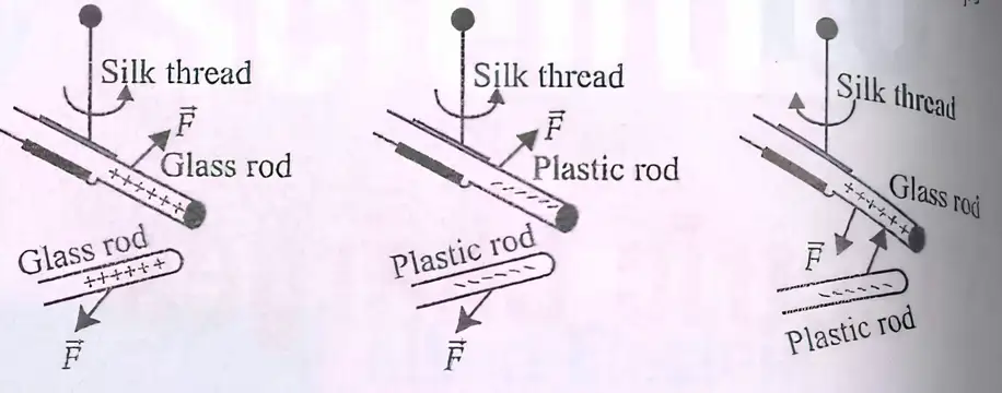
- Charge types: positive and negative. Like charges repel; unlike charges attract.
- Rubbing a glass rod or cat’s fur with silk or a plastic rod leaves the two objects with opposite charges.
- Charge convention: glass and cat’s fur are called positive; plastic and silk are called negative.
- Electrified or charged: an object that possesses electric charge is described as charged or electrified; an object with no net charge is neutral.
| Charges | Interaction |
|---|---|
| Like charges | Repel |
| Unlike charges | Attract |
Detecting Charge
- Gold-leaf electroscope: a simple instrument used to detect charge on a body.
Quick recap
- Electrostatics studies forces, fields and potentials arising from static electric charges.
- Electric-charge discharge through the body can cause a shock and is associated with the generation of static electricity.
- A neutral body becomes charged by gaining or losing electrons.
- Losing electrons makes an object positive; gaining electrons makes it negative.
- Like charges repel, while unlike charges attract.
- Rubbing glass or cat’s fur with silk or plastic leaves the objects with opposite charges; glass and fur are conventionally positive, while silk and plastic are negative.
- A gold-leaf electroscope detects charge on a body.
Conductors and Insulators
Conductors and Insulators
Insulator — A material that offers high resistance to the passage of electricity, so charge does not move freely through it.
| Point | Conductors | Insulators |
|---|---|---|
| Charge movement | Electrons move comparatively freely. | Charges do not move freely. |
| Electrical behaviour | Allow electricity to pass easily. | Offer high resistance to electricity. |
| Charge after transfer | Spreads over the entire surface. | Remains where it was transferred. |
| Examples | Metals, human and animal bodies, Earth | Glass, porcelain, plastic, nylon, wood |
Wires in Household Electric Wiring
- Live wire: Carries current from the power station to the electrical appliance.
- Neutral wire: Completes the circuit by carrying current back from the appliance.
- Earth wire: Connects the metal body of an appliance to the ground, carrying leakage charge safely away and helping prevent electric shock.
Quick recap
- Conductors allow electricity to pass easily because their electrons move comparatively freely.
- In conductors, transferred charge spreads over the entire surface.
- Insulators offer high resistance; transferred charge stays where it is placed.
- Live and neutral wires carry current from the power station.
- The earth wire connects metallic appliance bodies to the ground and carries extra charge away.
Basic Properties of Electric Charge
Addition of Charges
- Net charge: The total charge of a system is found by adding the charges of all its constituent bodies.
- Signed quantities: Positive and negative charges are added algebraically, so the net charge may be positive, negative or zero.
Conservation of Charge
- Isolated system: Its total electric charge remains constant over time.
- Transfer of charge: Charge may move from one body to another, but the total charge of the system is unchanged.
Quantisation of Charge
Charge in One Coulomb
- Electron count: A charge magnitude of corresponds to approximately elementary charges.
Quick recap
- The net charge of a system is the algebraic sum of its individual charges.
- The total charge of an isolated system remains constant.
- Charge is transferred, not created or destroyed.
- Charge is quantised: , where is a positive integer.
- The elementary charge is .
- A charge magnitude of contains about elementary charges.
Coulomb’s Law
Magnitude Form of Coulomb’s Law
Coulomb’s law — The magnitude of the electrostatic force between two point charges is proportional to the product of their magnitudes and inversely proportional to the square of their separation.
Here, is the distance between the charges, and is Coulomb’s constant.
Vacuum constants
- Permittivity of free space: .
- Coulomb’s constant: .
Vector Form and Force Direction
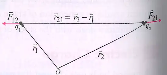
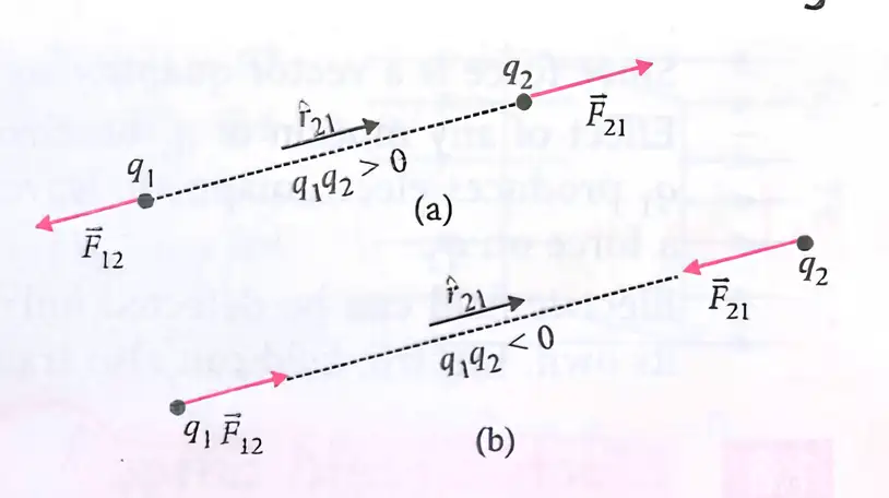
- Notation: is the force on due to ; points from to .
- Direction: The force acts along the line joining the charges; its direction depends on whether the charges are like or unlike.
is the force on due to ; the two forces are equal in magnitude and opposite in direction.
| Charge pair | Direction of | Interaction |
|---|---|---|
| Like charges | Along | Repulsion |
| Unlike charges | Along | Attraction |
Effect of a Dielectric Medium
Dielectric constant — is the dielectric constant of the medium; it reduces the force between charges compared with the force in vacuum.
is the force in vacuum; the medium reduces it by a factor of .
State Coulomb’s law for two point charges in vacuum.
How does a dielectric medium affect the Coulomb force?
Quick recap
- Coulomb’s law gives force proportional to and inversely proportional to .
- In vacuum, .
- The force acts along the line joining the two charges.
- Like charges repel; unlike charges attract.
- The forces on the two charges are equal and opposite: .
- A dielectric medium reduces the force to .
Forces Between Multiple Charges
Principle of Superposition
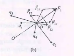
Principle of superposition — The net force on a charge due to several other charges equals the vector sum of the forces each charge produces individually.
Key points
- Calculate separately: Find the force on the chosen charge from each other charge, one at a time.
- Add as vectors: Include both magnitude and direction when combining the individual forces.
- No mutual alteration: The presence of other charges does not change each pairwise force.
Force on a Charge in a System of Many Charges
General form
- For charges: The force on is the sum of the forces on it due to charges through .
- Pairwise term: Each contribution follows Coulomb’s law and is directed along the line joining the two charges.
Quick recap
- The principle of superposition gives the net force as the vector sum of individual forces.
- Calculate each charge’s contribution separately using Coulomb’s law.
- Other charges do not alter the individual pairwise forces.
- For charges, sum the contributions from to to find the force on .
- Vector direction must be included when adding the forces.
Electric Field
Electric Field Due to a Point Charge
Electric field — A field is a quantity defined at every point in space whose value may vary from point to point; electric field at a point is the force per unit positive test charge placed there.
- Direction: The electric field points in the direction of the force on a positive test charge.
- Vector: Since force is a vector, electric field is also a vector.
Here, is the test charge, and points from the source charge to the field point.
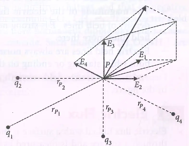
Electric Field Due to a System of Charges
Superposition principle
- Net force: The force on a test charge due to several point charges is the vector sum of the individual forces.
- Net field: The total electric field is the vector sum of the fields due to each source charge.
- Direction: For each charge, points from that charge to the field point .
Here, is the distance from charge to the field point.
Physical Significance of Electric Field
- Property of the source: The electric field is a characteristic of the system of charges and is independent of the test charge used to measure it.
- Propagation: A change in the motion of one charge does not affect another instantaneously; the accelerated charge produces electromagnetic waves that propagate at speed and can cause a force when they reach the other charge.
- Detection: An electric field is detected through its effects—the forces it exerts on charges.
- Dynamics and energy: The electric field has independent dynamics and can transport energy.
Quick recap
- A field is defined throughout space and may vary from point to point.
- Electric field is force per unit positive test charge and is a vector.
- A point charge produces a field given by .
- For multiple charges, net force and electric field are vector sums of individual contributions.
- Electric field is a property of the source charges, independent of the test charge.
- Electric effects propagate at speed ; fields are detected through forces and can transport energy.
Electric Field Lines
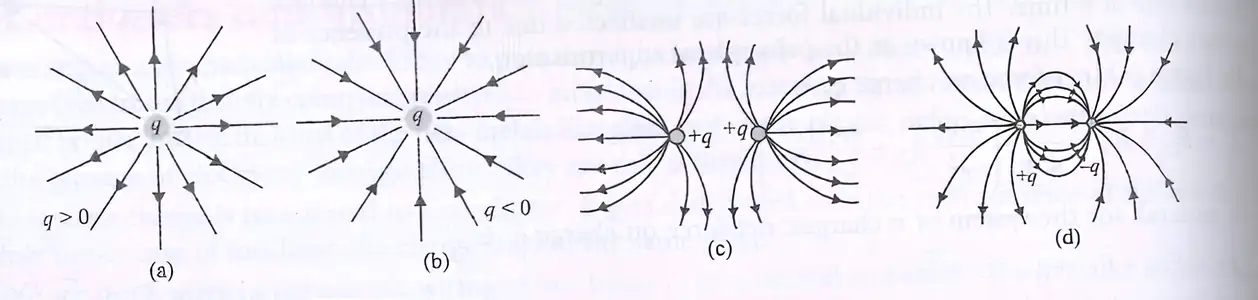
Electric field line — A curve whose tangent at any point gives the direction of the net electric field there.
Properties of Electric Field Lines
- Direction: The tangent to a field line at any point shows the direction of the electric field at that point.
- Continuity: Field lines are continuous; in a charge-free region, they have no breaks.
- Origins and ends: Lines start on positive charges and end on negative charges. For an isolated charge, they may start or end at infinity.
- No intersection: Two field lines cannot cross, because the field at one point cannot have two directions.
- No closed loops: Electrostatic field lines do not form closed loops, because the electrostatic field is conservative.
- Strength: Field-line density represents field magnitude; lines are denser where the field is stronger and more spread out where it is weaker.
- Conductors: Electric field lines meet a conductor’s surface perpendicularly, both where they start and where they end.
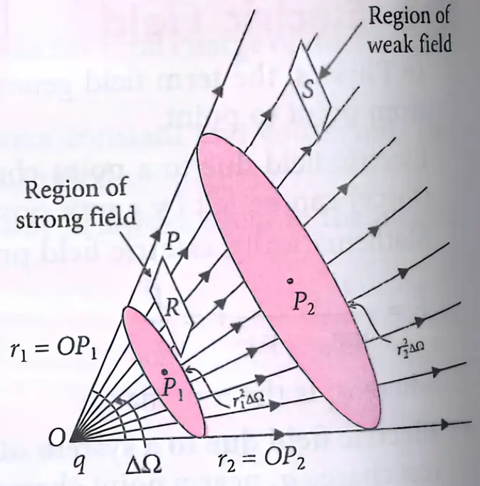
Do not interpret crossing field lines as a possible field pattern: an intersection would assign two directions to the electric field at the same point.
Quick recap
- An electric field line is tangent to the field direction at every point.
- Lines start on positive charges and end on negative charges, or at infinity for an isolated charge.
- Field lines are continuous and never intersect.
- Electrostatic field lines do not form closed loops.
- Greater field-line density indicates a stronger electric field.
- At a conductor’s surface, field lines are perpendicular.
Electric Flux
Electric flux — Electric flux measures the electric field passing through a surface and is the surface integral of the electric field over that surface.
Meaning and general expression
- Area vector: is normal to each small surface element; its magnitude is the element's area.
- Angle: is the angle between the electric field and the surface's area vector .
- General field: Flux through a surface is ; the dot product selects the field component normal to the surface.
- Uniform field: For a flat surface in a uniform electric field, .
Orientation, sign and units
- Field parallel to the surface: The field is perpendicular to the area vector, so and .
- Field normal to the surface: The field is parallel to the area vector, so and the flux is maximum: .
- Scalar: Electric flux is a scalar quantity; its sign depends on the direction of the field relative to the area vector.
- SI units: Electric flux is measured in , equivalently .
Flux and electric field
- Zero flux: Electric field can be non-zero even when the net flux through a surface is zero.
- Non-zero flux: Non-zero electric flux requires a non-zero electric field component through the surface.

Quick recap
- Electric flux measures the electric field passing through a surface.
- The area vector is perpendicular to the surface; flux depends on the field component along it.
- For a uniform field, ; in general, .
- Flux is zero when the field is parallel to the surface and maximum when the field is normal to it.
- Electric flux is a scalar measured in or .
- Zero flux does not necessarily mean the electric field is zero.
Electric Dipole
Electric Dipole and Dipole Moment
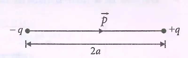
Electric dipole — A pair of equal and opposite charges separated by a small distance.
Dipole moment
- Magnitude: For charges and separated by , the dipole moment is .
- Direction: The vector points from the negative charge to the positive charge.
- SI unit: Coulomb-metre ().
Here, is directed from to .
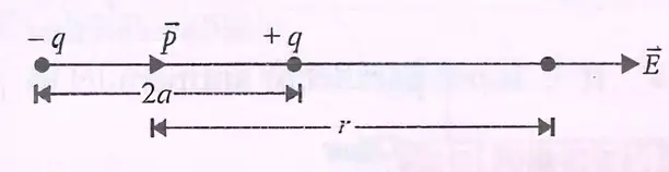
Electric Field on the Dipole Axis
Axial or end-on position
- Exact field: At an axial point a distance from the dipole centre, the net field is along .
- Far-field approximation: When , the axial field decreases as .
For an axial point outside the dipole, .
Use when .
Electric Field on the Equatorial Line
Equatorial or broadside-on position
- Direction: The net field is opposite to the dipole moment, .
- Far-field approximation: When , the magnitude decreases as .
The negative sign indicates a direction opposite to .
Use when .
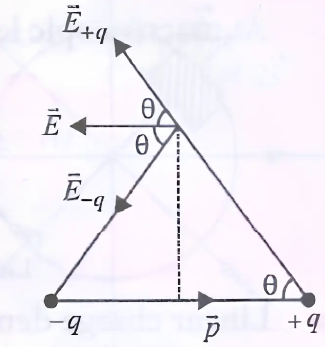
| Point | Axial | Equatorial |
|---|---|---|
| Direction | Along | Opposite to |
| Magnitude | ||
| Ratio | The axial field is twice the equatorial field in magnitude. |
Dipoles in Molecules
Permanent and induced dipoles
- Non-polar molecules: Positive and negative charge centres coincide, so there is no permanent dipole moment; examples include and .
- Induced dipole: An applied electric field can separate the charge centres of a non-polar molecule and produce a dipole moment.
- Polar molecules: Their positive and negative charge centres do not coincide, so they have a permanent dipole moment; examples include and .
Electric Field at a General Point
Short dipole approximation
- Setup: For a short dipole, take point at distance from its centre and at angle to the dipole axis, with .
- Resolution: Resolve into along the end-on direction and along the broadside-on direction.
- Components: The field components have magnitudes and , where .
- Resultant: The components are perpendicular; combine them to find the field magnitude and its angle to .
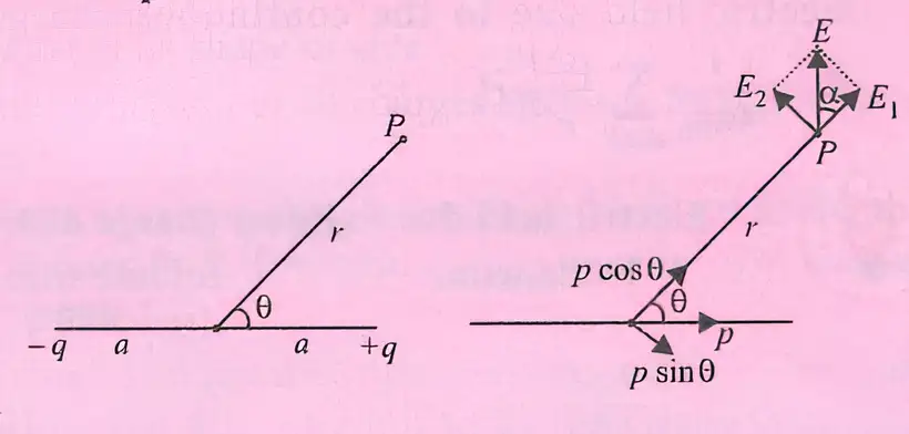
Here, .
Obtained from .
The angle is measured between and .
Do not confuse the field directions: the axial field is along , while the equatorial field is opposite to .
What is the dipole moment of charges and separated by distance ?
At large distances, how do the axial and equatorial fields compare?
Quick recap
- A dipole consists of equal, opposite charges; points from negative to positive charge.
- The far axial field is along .
- The far equatorial field is opposite to .
- At large distance, the axial field magnitude is twice the equatorial field magnitude.
- Polar molecules have permanent dipole moments; non-polar molecules can acquire induced dipoles in an electric field.
- For a short dipole, .
Dipole in a Uniform External Field
Dipole in a Uniform Electric Field
| Angle between and | Torque magnitude |
|---|---|
| or | Minimum: |
| Maximum: |
Dipole in a Non-uniform Electric Field
- Non-uniform field: The electric field varies in magnitude or direction from point to point.
- Net force: The forces on the two charges of a dipole may not cancel, so the dipole can experience a net force as well as a torque.
Oscillation of a Dipole in a Uniform Field
Here, is the dipole’s moment of inertia, is its dipole moment, and is the uniform field strength.
Why is the net force on a dipole zero in a uniform electric field, even though it can experience torque?
Quick recap
- A dipole in a uniform electric field has zero net force.
- Its torque magnitude is , with vector form .
- Torque is zero when is parallel or antiparallel to , and maximum when perpendicular.
- A non-uniform field can exert a net force on a dipole; a non-aligned dipole also experiences torque.
- The oscillation period is for small angular oscillations.
Continuous Charge Distribution
Continuous charge distribution — At the macroscopic level, charge is treated as continuously spread because the concentration of electrons is very high.
Charge Densities
| Distribution | Density | Definition | SI unit |
|---|---|---|---|
| Linear | Charge per unit length: | ||
| Surface | Charge per unit area: | ||
| Volume | Charge per unit volume: |
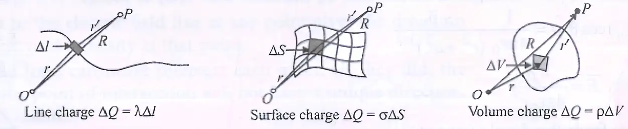
Electric Field of a Continuous Distribution
- Charge element: Divide the distribution into small elements, each carrying a small charge.
- Total field: Add the electric-field contributions of all charge elements as vectors.
Sum the contributions of the small charge elements; in the continuous limit, use an integral.
Use the charge element matching the geometry of the distribution.
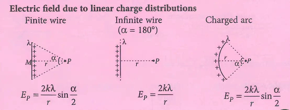
Electric Field Due to Linear Charge Distributions
For a uniformly charged finite wire, with the observation point a perpendicular distance away and endpoint angles and measured from the perpendicular, the net field is perpendicular to the wire when the perpendicular foot lies between its ends.
At perpendicular distance from a uniformly charged infinite wire, the field is radial and has magnitude:
For an arc of radius , linear density , and total angle , the field at the centre lies along the arc's symmetry axis, toward the open side for positive charge.
Field on the Axis of a Charged Ring
- Geometry: A ring of radius has total charge ; point lies on its axis at distance from the centre.
- Symmetry: Transverse components from opposite ring elements cancel; only axial components add.
- Distance: Every ring element is at distance from .
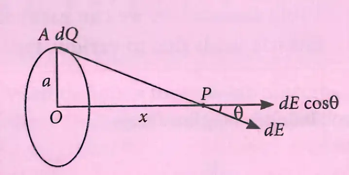
The element's field has magnitude ; only its axial component contributes to the net field.
Integrating around the ring gives the net axial field. For positive and , it points away from the ring along the axis.
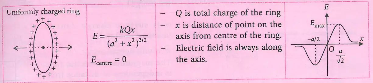
Do not add field magnitudes directly for a continuous distribution; add vector contributions, or use symmetry to cancel components first.
Quick recap
- At macroscopic scales, charge distributions can be treated as continuous.
- Linear, surface and volume charge densities are charge per length, area and volume, respectively.
- Find the field by adding the vector contributions of small charge elements.
- For an infinite wire, ; finite-wire and arc fields depend on their geometry.
- On a charged ring's axis, transverse components cancel and the net field is axial.
- The ring's axial field is .
Gauss’s Law
Gauss’s law — The total electric flux through any closed surface in vacuum equals the net charge enclosed divided by the permittivity of free space.
The integral is taken over a closed surface; is the net charge inside it.
Key points
- Any shape or size: Gauss’s law holds for every closed surface.
- Enclosed charge: Count the algebraic sum of all charges inside the surface; their positions within it do not matter.
- External charges: Charges outside the surface can contribute to the electric field on it, but not to .
- Gaussian surface: This is the chosen closed surface used to apply Gauss’s law.
- Discrete charges: Do not let the Gaussian surface pass through a discrete charge, where its electric field is not well-defined; it may pass through a continuous charge distribution.
Spherical surface around a point charge
Verification for a charge at the centre
- Symmetry: For a point charge at the centre of a sphere of radius , the electric field is radial and has the same magnitude everywhere on the sphere.
- Flux: The field and outward area vector are parallel, so .
- Field magnitude: On the sphere, .
- Result: Multiplying the field by the sphere’s area, , gives , as Gauss’s law states.
Here is constant over the sphere and .
Field magnitude at distance from charge .
Substituting the point-charge field into the spherical flux expression cancels the radius dependence.
Uses and significance
- Symmetry: Gauss’s law can simplify electric-field calculations when the charge distribution has suitable symmetry.
- Underlying dependence: The law relies on the inverse-square dependence of the electric field in Coulomb’s law.
- Implication: A violation of Gauss’s law would indicate a departure from the inverse-square law.
Do not include external charges in : they may affect the field on the surface, but only charges inside determine the net flux.
What determines the net electric flux through a closed Gaussian surface?
Quick recap
- Gauss’s law relates the total flux through a closed surface to the net enclosed charge.
- The law applies to closed surfaces of any shape or size.
- External charges can affect the field on a surface, but they are excluded from enclosed charge.
- A Gaussian surface is chosen for applying the law and must not pass through a discrete charge.
- For a point charge at a sphere’s centre, the flux is .
- Gauss’s law is especially useful for electric-field calculations with symmetry.
Application of Gauss’s Law
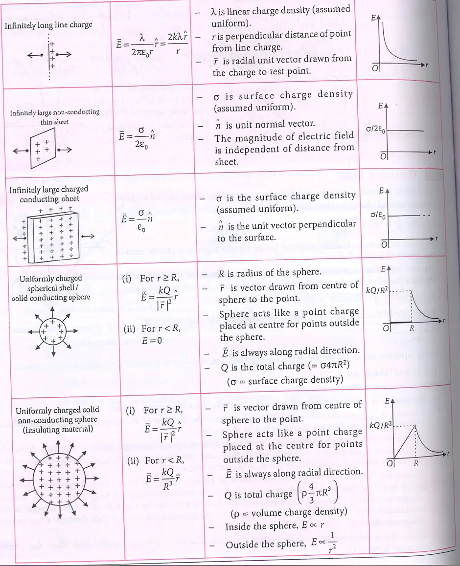
Using Gauss’s Law
Application of Gauss’s law — Gauss’s law can be used to find electric fields for some charge configurations.
Electric fields for charge distributions
- Charge distributions: Electric fields can be considered for various types of charge distribution.
- Patterns and distance: Field patterns and how the field depends on distance differ among charge distributions.
Quick recap
- Gauss’s law can help find electric fields for some charge configurations.
- Electric fields are considered for various types of charge distribution.
- Field patterns vary among charge distributions.
- The distance dependence of the field is also shown for common charge distributions.
NEET Physics — ALL CHAPTERS
1
Basic Mathematics
2
Units and Measurement
3
Motion in a Straight Line
4
Motion in a Plane
5
Laws of Motion
6
Work, Energy and Power
7
System of Particles and Rotational Motion
8
Gravitation
9
Mechanical Properties of Solids
10
Mechanical Properties of Fluids
11
Thermal Properties of Matter
12
Thermodynamics
13
Kinetic Theory
14
Oscillations
15
Waves
16
Electric Charges and Fields
17
Electrostatic Potential and Capacitance
18
Current Electricity
19
Moving Charges and Magnetism
20
Magnetism and Matter
21
Electromagnetic Induction
22
Alternating Current
23
Electromagnetic Waves
24
Ray Optics and Optical Instruments
25
Wave Optics
26
Dual Nature of Radiation and Matter
27
Atoms
28
Nuclei
29
Semiconductor Electronics: Materials, Devices and Simple Circuits