NEET UG . NEET Physics . Physics . Magnetism and Matter
Chapter 20: Magnetism and Matter
Ch 20
NEET Physics
NEET UG
The Bar Magnet
Basic Ideas of Magnetism
- Magnetism: Magnets attract materials such as iron, nickel and cobalt.
- Magnetic poles: Like poles repel and unlike poles attract; magnetic poles always occur in pairs.
The Bar Magnet
- Poles: The ends of a bar magnet, where its magnetic force is strongest, are called its poles.
- Alignment: A freely suspended bar magnet points approximately north–south; its north-seeking end is the north pole.
- Dipole: A bar magnet has both poles, which cannot be isolated by breaking the magnet.
Magnetic Field Lines
- Direction: The tangent to a magnetic field line at any point gives the direction of the magnetic field there.
- Strength: A greater density of field lines indicates a stronger magnetic field.
- Properties: Magnetic field lines form closed continuous loops and never intersect.
Bar Magnet as an Equivalent Solenoid
- Similarity: A bar magnet and a finite solenoid produce similar magnetic fields.
- Far axial field: For a short bar magnet, the field at an axial point far away is approximately , where is its magnetic dipole moment.
A Magnetic Dipole in a Uniform Field
This is the work-related potential energy for a dipole oriented at angle to the field; it is zero at .
| Physical quantity | Electrostatics | Magnetism |
|---|---|---|
| Dipole moment scaling | ||
| Equatorial field of a short dipole | ||
| Axial field of a short dipole | ||
| Torque in an external field | ||
| Potential energy in an external field |
Why is repulsion the surest test for identifying a magnet?
State two properties of magnetic field lines.
Write the torque and potential energy of a magnetic dipole in a uniform magnetic field.
Quick recap
- A magnet attracts materials such as iron, nickel and cobalt; a freely suspended bar magnet aligns north–south.
- Like poles repel and unlike poles attract; magnetic poles always occur in pairs.
- Every broken piece of a bar magnet remains a dipole with both poles.
- Magnetic field lines are closed, non-intersecting loops; their tangent and density show direction and strength.
- A bar magnet has far axial field and resembles a finite solenoid.
- A dipole in a uniform field experiences torque and has potential energy .
Magnetism and Gauss’s Law
Magnetic Flux and Gauss’s Law
Use the dot product to account for the angle between the field and the surface normal.
Gauss’s law of magnetism — The net magnetic flux through any closed surface is zero.
Magnetic Poles
- No monopoles: Isolated magnetic poles do not exist; magnets have no separate magnetic source or sink.
- Simplest magnetic element: A magnetic dipole or a current loop.
Zero net flux does not mean the magnetic field is zero everywhere on the surface; incoming and outgoing flux cancel.
Quick recap
- Magnetic flux through a surface depends on the field’s angle to the surface normal.
- The net magnetic flux through any closed surface is zero.
- Flux entering a closed surface equals flux leaving it.
- Magnetic monopoles do not exist; magnetic fields have no isolated sources or sinks.
- A dipole or current loop is the simplest magnetic element.
Magnetisation and Magnetic Intensity
Magnetising Field Intensity
Magnetising field intensity — The vector field expresses the ability of a magnetic field to magnetise a material.
- Nature: is a vector quantity.
- SI unit: .
- Field relation: Magnetic induction in a medium is related to magnetising field by , where is the medium's permeability.
Intensity of Magnetisation
Intensity of magnetisation — The net magnetic dipole moment per unit volume of a magnetised material is its intensity of magnetisation, .
- Nature: is a vector quantity.
- SI unit: ; dimensional formula: .
- Uniform bar specimen: For cross-sectional area , magnetic length and pole strength , its magnetic moment is and its volume is .
Magnetic Susceptibility
Magnetic susceptibility — Magnetic susceptibility, , is the ratio of intensity of magnetisation to magnetising field.
- Nature: Scalar quantity.
- Units and dimensions: Dimensionless; it has no unit.
- Meaning: Indicates how strongly a material responds to an external magnetic field.
Magnetic Permeability
Magnetic permeability — Permeability, , is the ratio of magnetic induction to magnetising field intensity in a medium.
- Nature: Scalar quantity.
- SI unit: ; dimensional formula: .
- Meaning: Measures the extent to which a medium permits a magnetic field to penetrate it.
Relative Permeability
Relative permeability — Relative permeability, , is the ratio of a medium's permeability to the permeability of free space, .
- Units and dimensions: Dimensionless; it has no unit.
Permeability–Susceptibility Relation
- Linear material: When magnetised by field intensity , a material's magnetic induction is .
- Also: Since , equating the two expressions gives the permeability–susceptibility relation.
Quick recap
- Magnetising field intensity describes a field's ability to magnetise a material.
- Intensity of magnetisation is magnetic moment per unit volume; for a uniform bar, .
- Susceptibility is and has no units or dimensions.
- Permeability is , with SI unit .
- Relative permeability is and is dimensionless.
- For a linear material, and .
Magnetic Properties of Materials
Classification of Magnetic Materials
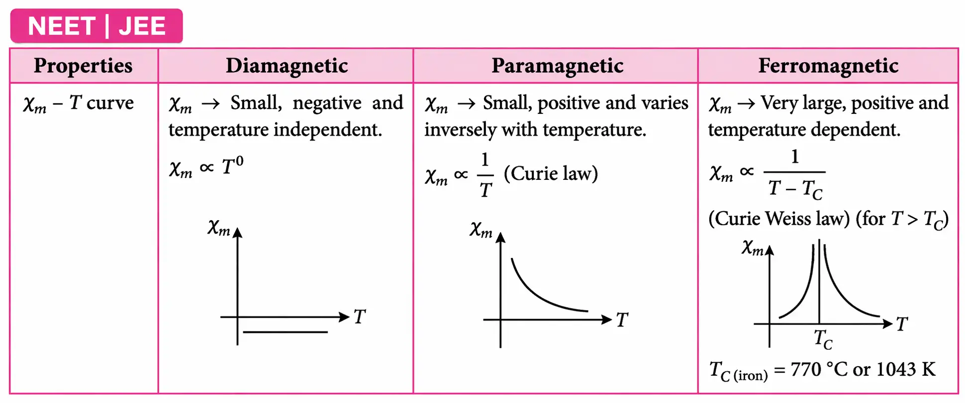
Magnetic susceptibility — Magnetic susceptibility, , indicates a material's response to an applied magnetic field; materials are classified using it, intensity of magnetisation , and relative permeability .
| Property | Diamagnetic | Paramagnetic | Ferromagnetic |
|---|---|---|---|
| Cause of magnetism | Orbital motion of electrons | Electron spin | Formation of magnetic domains |
| Response in a uniform field | Weak magnetisation opposite to the field; | Weak magnetisation along the field; | Strong magnetisation along the field; |
| – behaviour | Small negative ; linear with negative slope | Small positive ; linear with positive slope | Large positive ; nonlinear increase that levels off |
| Relative permeability | ; | ; | ; |
| Atomic magnetic moments | No permanent magnetic moment | Permanent moments, randomly oriented without an external field | Permanent moments organised into domains |
| Examples | Bismuth, copper, lead, water, sodium chloride | Aluminium, sodium, calcium, oxygen, copper chloride | Iron, cobalt, nickel, gadolinium |
Magnetic Field of a Bar Magnet
Notation
- Pole strength: Let each pole have strength and lie a distance from the magnet's centre.
- Magnetic moment: The magnet's moment is ; denotes the distance from its centre.
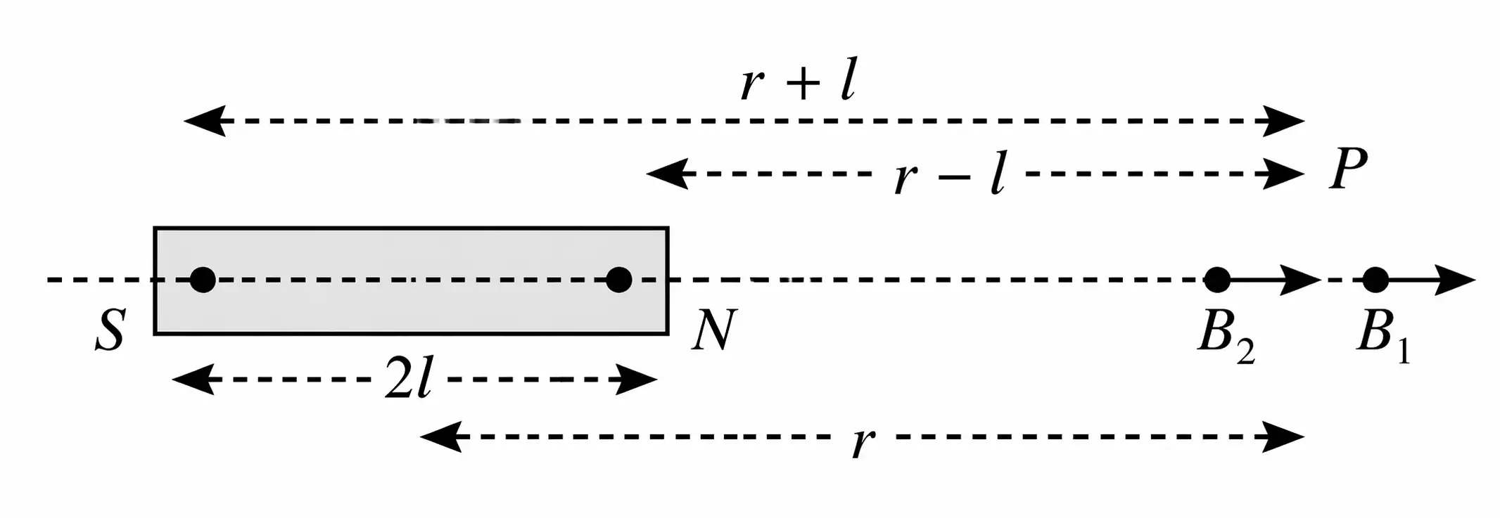
Axial position
- Pole contributions: The north-pole field points away from the north pole; the south-pole field points toward the south pole. At an external axial point, they oppose, and the nearer pole's field is stronger.
- Net direction: The resultant axial field points along the magnet's magnetic moment.
For an external axial point, .
For a short magnet, ; the field has the form of a dipole field.
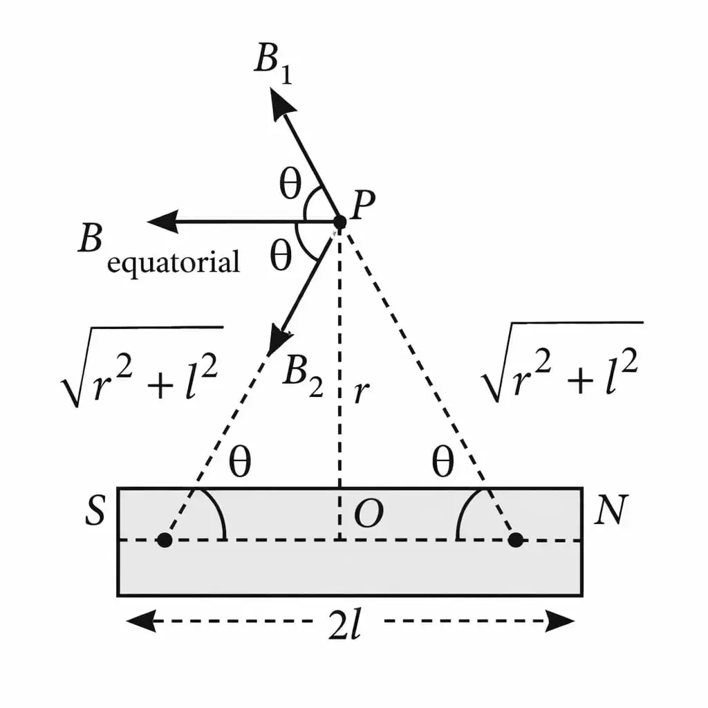
Equatorial position
- Distance to each pole: For an observation point on the equatorial line, the distance to either pole is .
- Net direction: The resultant field is opposite to the magnet's magnetic moment.
This is the magnitude of the field.
For .
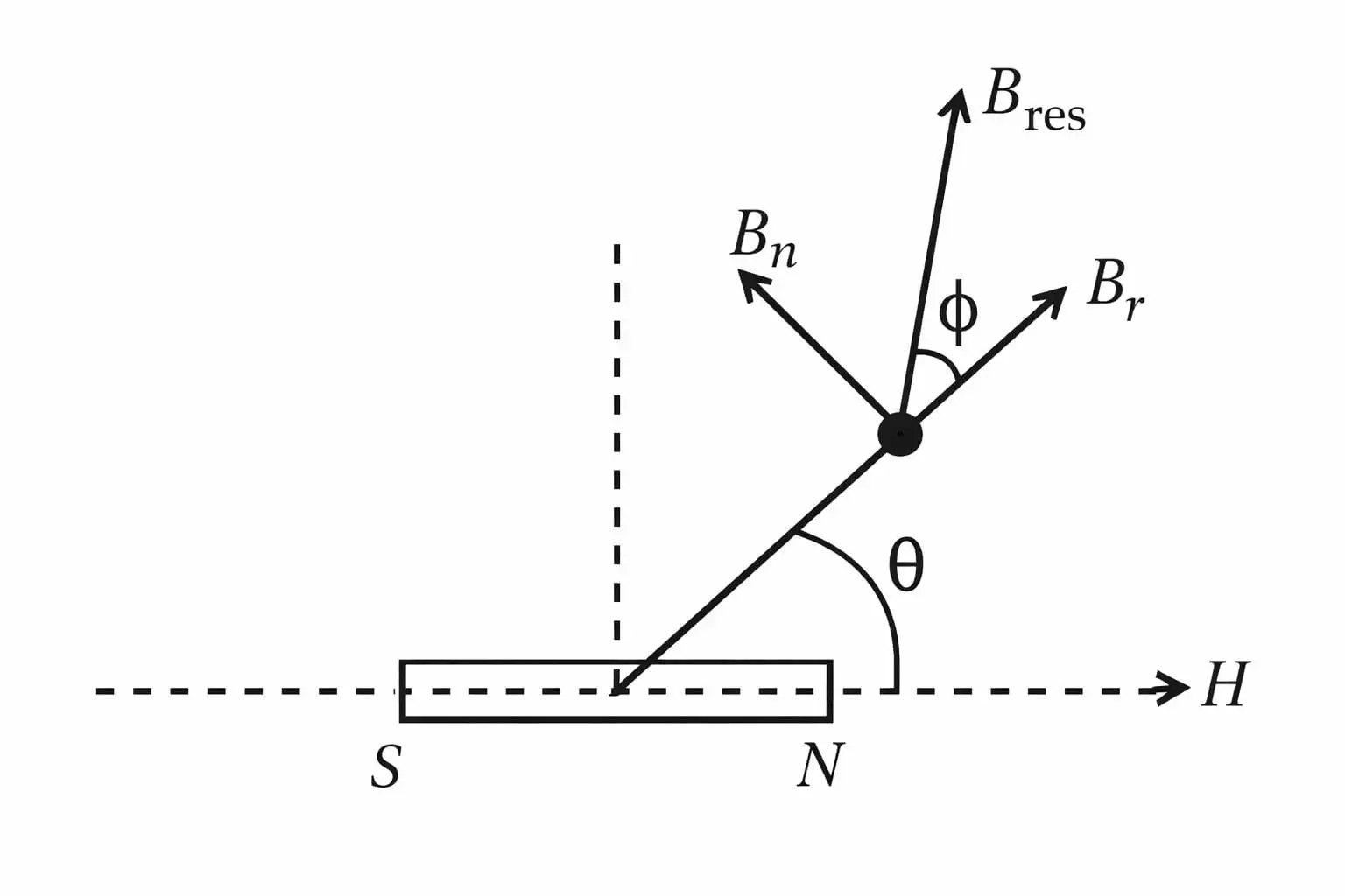
General position
- Position angle: Let be the angle between the position vector and the magnetic axis.
- Components: The field components are radial, , and perpendicular to the radial direction, .
The resultant field magnitude is ; is the angle between the resultant field and the radial direction.
Magnetic Hysteresis
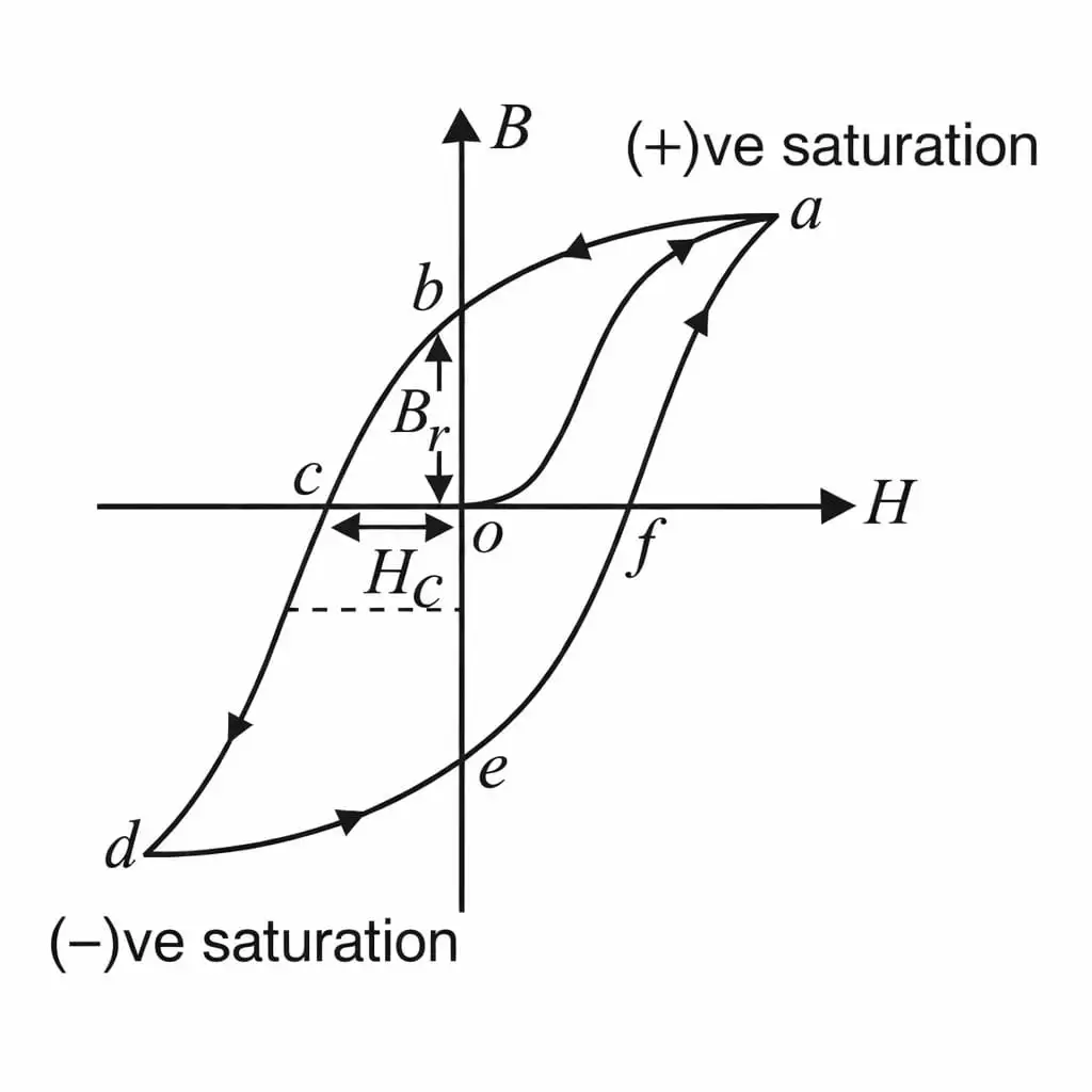
Magnetic hysteresis — Magnetic hysteresis is the lag of magnetic induction behind the magnetising field during magnetisation and demagnetisation of a ferromagnetic material.
Hysteresis loop and terms
- Loop formation: As increases, rises nonlinearly towards saturation; when returns to zero, follows a different path.
- Cause: When the external field is removed, some domains remain aligned in the previous direction, leaving residual magnetism.
- Retentivity (remanence): The residual induction when the magnetising field is reduced to zero.
- Coercivity: The reverse magnetising field required to destroy the residual magnetism.
| Property | Soft ferromagnetic material | Hard ferromagnetic material |
|---|---|---|
| Hysteresis loop | Narrow | Wide |
| Coercivity | Low; readily demagnetised | High; resists demagnetisation |
| Retentivity | Lower | Higher |
How do diamagnetic, paramagnetic, and ferromagnetic materials respond to an applied field?
Define retentivity and coercivity.
Quick recap
- Diamagnetic materials magnetise weakly opposite to the applied field; paramagnetic materials weakly along it; ferromagnetic materials strongly along it.
- A bar magnet has moment ; its short-magnet axial and equatorial fields vary as .
- The short-magnet axial field magnitude is twice the equatorial field magnitude.
- At an equatorial point, the magnetic field points opposite to the magnet's moment.
- Magnetic hysteresis is the lag of behind in ferromagnetic materials, caused by domains that remain aligned.
- Retentivity measures residual induction; coercivity measures the reverse field needed to remove residual magnetism.
NEET Physics — ALL CHAPTERS
1
Basic Mathematics
2
Units and Measurement
3
Motion in a Straight Line
4
Motion in a Plane
5
Laws of Motion
6
Work, Energy and Power
7
System of Particles and Rotational Motion
8
Gravitation
9
Mechanical Properties of Solids
10
Mechanical Properties of Fluids
11
Thermal Properties of Matter
12
Thermodynamics
13
Kinetic Theory
14
Oscillations
15
Waves
16
Electric Charges and Fields
17
Electrostatic Potential and Capacitance
18
Current Electricity
19
Moving Charges and Magnetism
20
Magnetism and Matter
21
Electromagnetic Induction
22
Alternating Current
23
Electromagnetic Waves
24
Ray Optics and Optical Instruments
25
Wave Optics
26
Dual Nature of Radiation and Matter
27
Atoms
28
Nuclei
29
Semiconductor Electronics: Materials, Devices and Simple Circuits