NEET UG . NEET Physics . Physics . Moving Charges and Magnetism
Chapter 19: Moving Charges and Magnetism
Ch 19
NEET Physics
NEET UG
Magnetic Force
Magnetic Fields and Their Representation
Magnetic fields
- Source: Electric currents and moving charges produce a magnetic field, represented by the vector .
- Superposition: The net magnetic field from several sources is the vector sum of the fields produced by each source.
- Current in a straight wire: Compass needles align tangentially to circles centred on the wire.
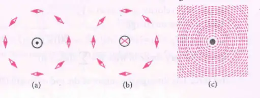
| Symbol | Meaning |
|---|---|
| Direction emerging out of the page | |
| Direction going into the page |
Lorentz Force on a Moving Charge
Lorentz force — The total force on a charge moving in electric and magnetic fields is the sum of its electric and magnetic forces.
The magnetic part is .
Here is the angle between and .
| Condition | Magnetic force |
|---|---|
| Maximum: | |
| or antiparallel | Zero: |
| Zero; a stationary charge experiences no magnetic force |
Direction of magnetic force
- Right-hand rule: For a positive charge, the force direction follows .
- Negative charge: Its force is opposite to the direction given by .
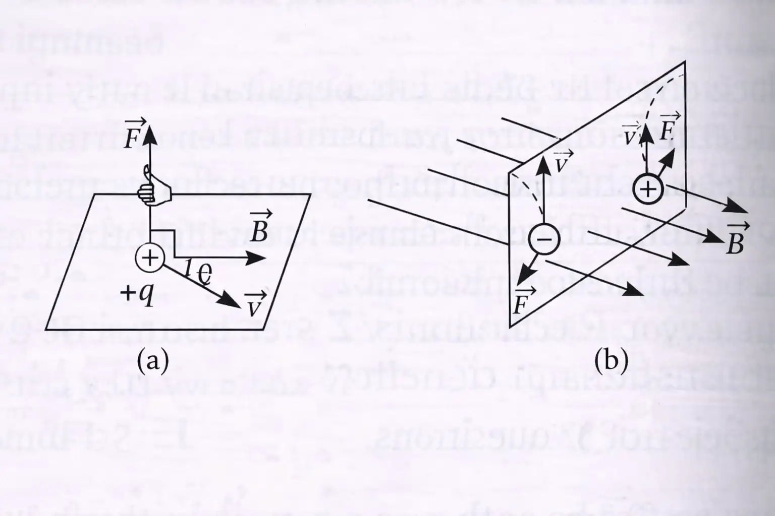
The magnetic-force relation defines the SI unit of magnetic field: tesla ().
Force on a Current-Carrying Conductor
From moving charges to current
- Charge carriers: In a wire segment of length and cross-sectional area , the number of mobile carriers is , where is the number density.
- Current density: The current density has magnitude , where is the carrier charge magnitude and is drift speed.
- Force: Adding the magnetic forces on the carriers gives the force on a straight conductor in a uniform magnetic field.
Here points along the conventional current; the force is perpendicular to both current direction and field.
For a curved or non-uniformly oriented wire, add the force contributions along its elements.
Force on a current-carrying rod
- Uniform rod: In a uniform field, the resultant force on a straight rod acts through its centre.
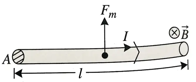
When is the magnetic force on a moving charge maximum and when is it zero?
Write the magnetic force on a straight current-carrying conductor.
Quick recap
- Currents and moving charges produce vector magnetic fields; fields from multiple sources add vectorially.
- Magnetic force on a charge is .
- Its magnitude is ; it is greatest at and zero at or .
- Positive and negative charges experience magnetic forces in opposite directions.
- The SI unit of magnetic field is the tesla, and .
- A straight current-carrying conductor experiences .
Motion in a Magnetic Field
Effect of the Angle Between Velocity and Magnetic Field
- Angle: The particle’s path depends on the angle between its velocity and the magnetic field.
- Parallel motion: When velocity is parallel or antiparallel to the field, magnetic force is zero and the particle travels in a straight line.
- Oblique motion: When velocity has both parallel and perpendicular components, the particle follows a helical path.
Circular Motion: Velocity Perpendicular to the Field
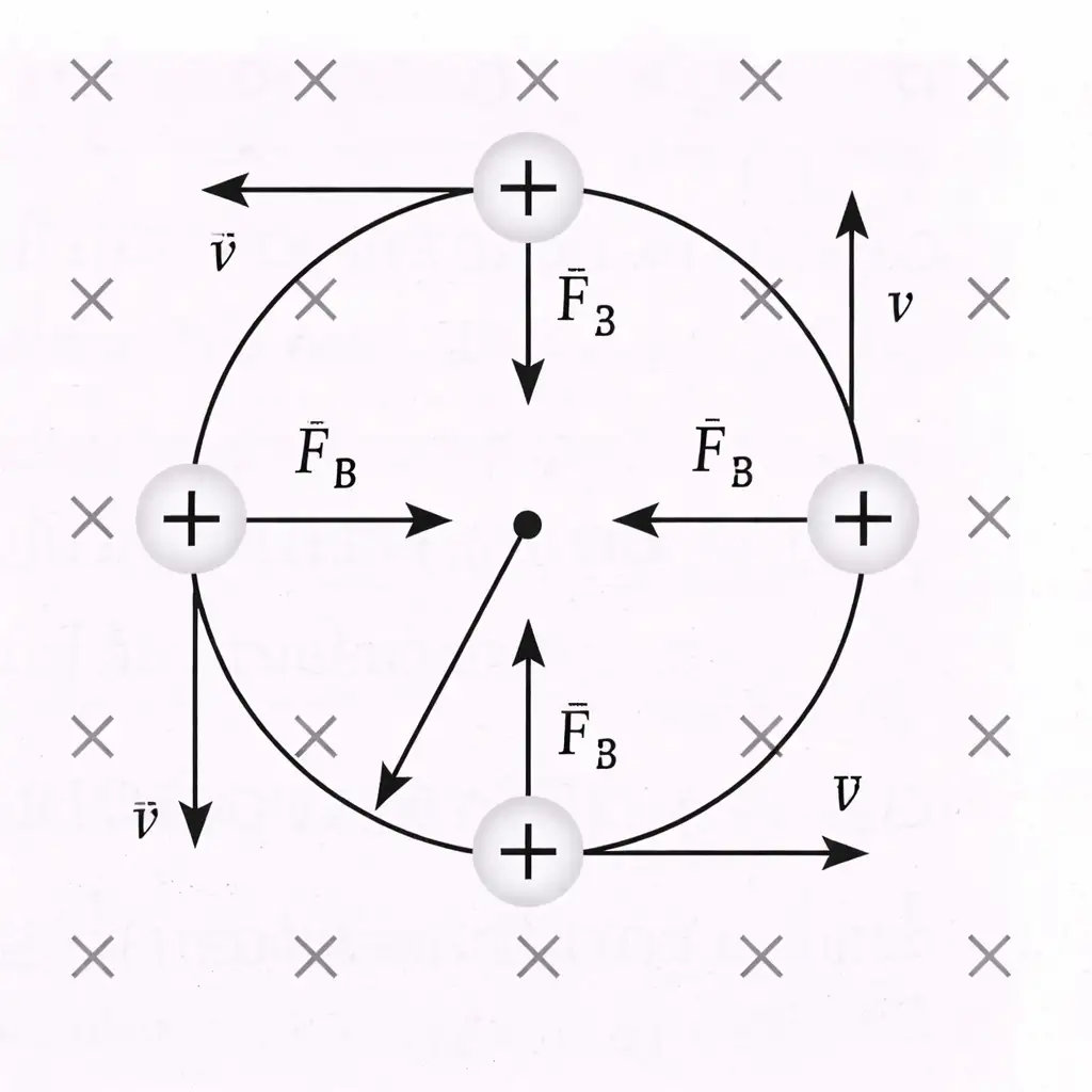
Radius, Period and Frequency
- Centripetal force: Equating magnetic force with centripetal force gives the radius of the circular orbit.
- Momentum form: Here is linear momentum and is kinetic energy; the radius depends on momentum and magnetic field.
Use the magnitude of the charge for the orbit radius.
These quantities depend on the magnetic field and the particle’s specific charge, not on its speed or orbit radius.
Do not assume that the period changes with speed or orbit radius: is independent of both and depends on , and .
Helical Motion: Velocity at an Angle to the Field
Velocity Components and Path
- Parallel component: remains constant and carries the particle along the field.
- Perpendicular component: causes circular motion around the field direction.
- Result: The combined motion is a helix; its circular plane is perpendicular to the field, and its axis is parallel to the field.
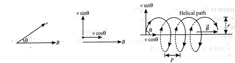
The perpendicular velocity component sets the circular radius; the revolution period is unchanged from the perpendicular-motion case.
Pitch is the distance travelled parallel to the field during one revolution.
Deviation in a Finite Magnetic-Field Region
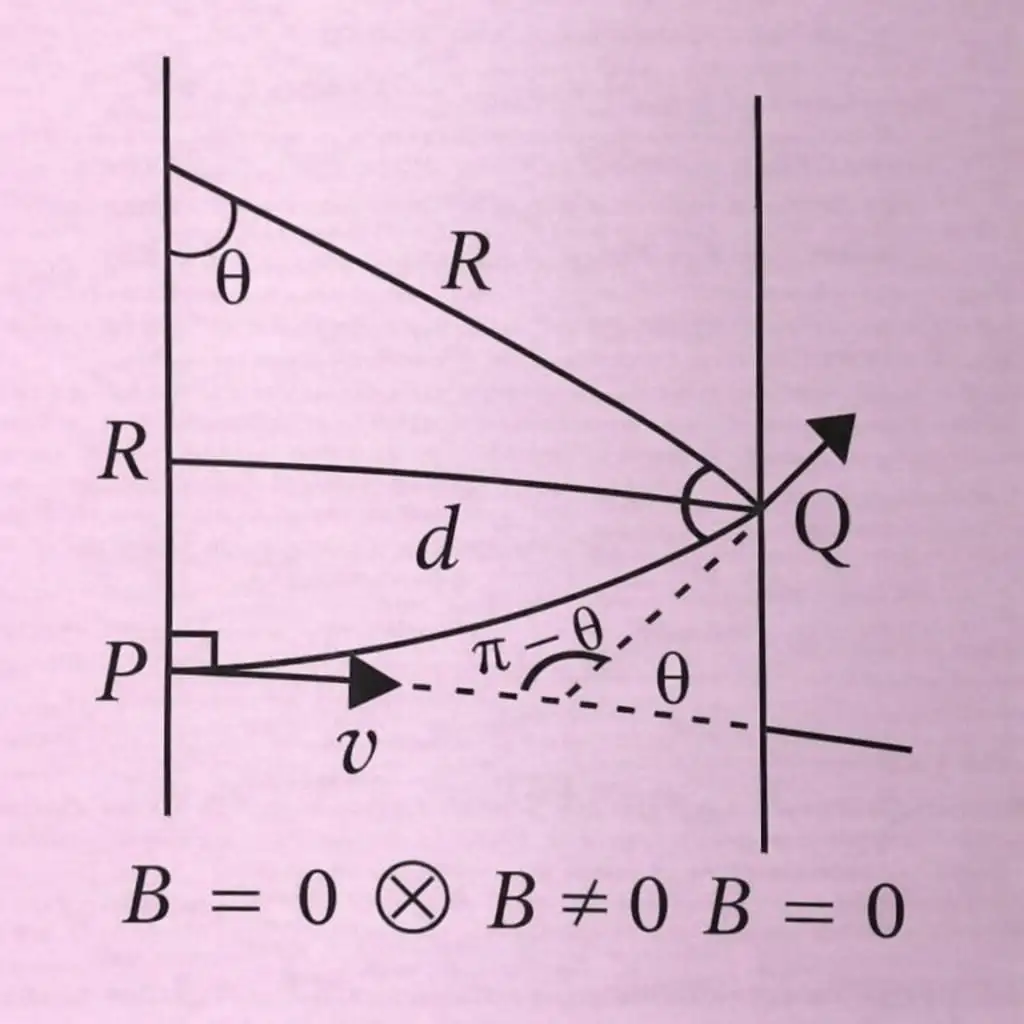
Particle Path Through a Field Region
- Inside the field: A particle entering a uniform field follows a circular arc of radius .
- Outside the field: After leaving the field, it travels in a straight line tangent to the circular path.
- Deviation angle: For field width , the geometry gives .
- Larger width: If , the deviation angle is .
Why is the speed of a charged particle unchanged in a magnetic field?
What determines the radius and pitch of a helical path?
Quick recap
- Parallel or antiparallel motion: No magnetic force; the path is straight.
- Perpendicular motion: The magnetic force supplies centripetal force, producing a circle.
- Circular radius: ; the period is .
- Cyclotron frequency: , independent of speed and orbit radius.
- Oblique motion: Parallel velocity stays constant while perpendicular velocity produces a helix.
- Helix measures: Radius depends on ; pitch is .
- Finite field region: For , ; for , .
Magnetic Field Due to a Current Element , Biot-Savart Law
Biot–Savart Law
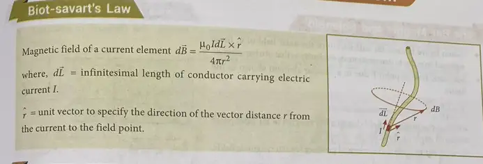
Biot–Savart law — The magnetic field contribution from a small current element depends on its distance and orientation relative to the field point.
Magnitude and direction
- Magnitude: , where is the angle between and .
- Vector form: .
- Direction: is perpendicular to the plane containing and ; determine it using the right-hand rule.
- Free-space permeability: .
| Point | Biot–Savart law | Coulomb’s law |
|---|---|---|
| Source | Vector current element | Scalar electric charge |
| Distance dependence | Varies as | Varies as |
| Direction | Perpendicular to the plane containing and | Along the displacement vector from source to field point |
| Angle dependence | Depends on ; the field is zero along the current-element direction | No corresponding angular factor |
The permeability and permittivity of free space are related through the speed of light in vacuum.
Field Due to a Finite Straight Current-Carrying Wire
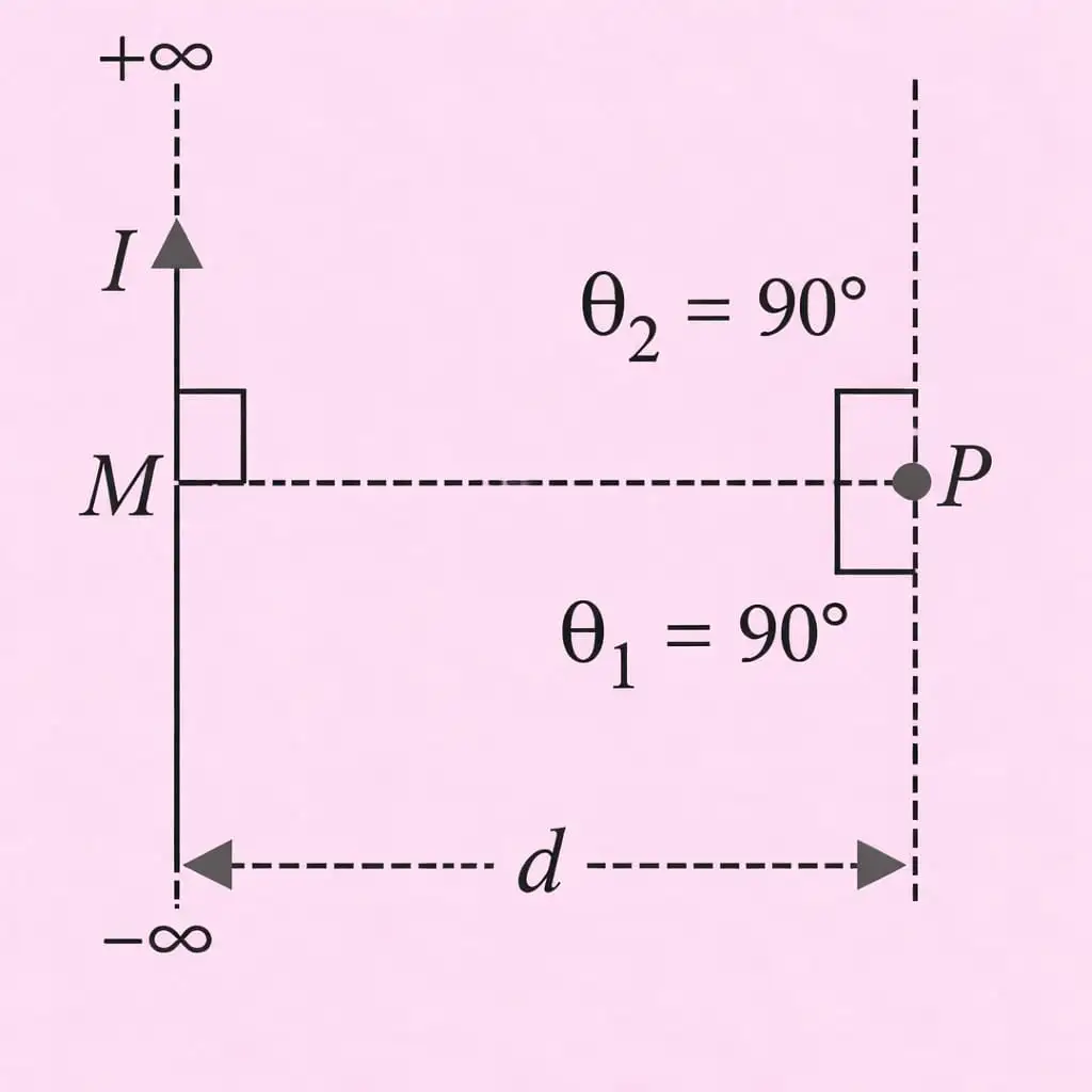
Geometry and integration
- Geometry: Let be the perpendicular distance from the wire to point , and let describe the position of a wire element relative to the perpendicular.
- Element contribution: The angle between and is , so .
- Geometry relations: , hence ; also .
- Direction: In the illustrated arrangement, all element contributions at point inward, so their magnitudes add.
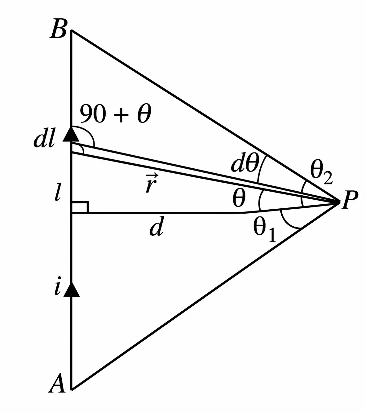
Integrate the contributions between endpoint angles and .
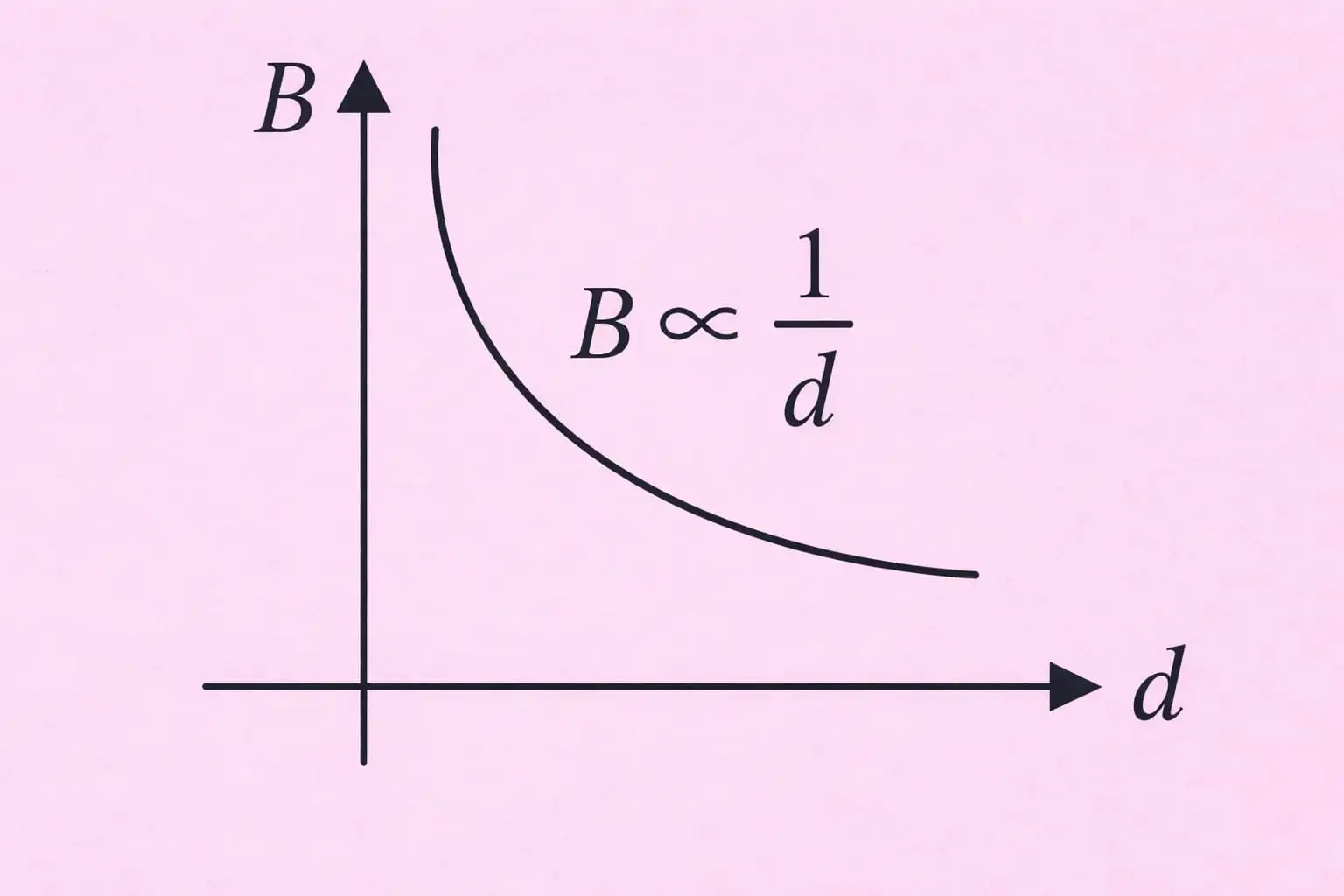
Infinite and Semi-Infinite Straight Wires
The lecture labels this result as the magnetic field at due to a semi-infinite wire.
State the Biot–Savart law in vector form and give the direction of .
Write the magnetic field due to a finite straight wire in terms of its endpoint angles.
What field result does the lecture state for the semi-infinite wire at distance ?
Quick recap
- Biot–Savart law: .
- The field direction is perpendicular to the plane containing the current element and position vector.
- For a finite straight wire, .
- The lecture states for the wire case labeled semi-infinite.
- Free-space constants obey .
Magnetic Field on the Axis of a Circular Current Loop
Field on the Loop Axis
Biot–Savart law — The magnetic field due to a current element depends on its current, length, orientation, and distance from the observation point.
Here, points from the current element to the observation point, and .
Applying the Law to a Circular Loop
- Geometry: For a loop of radius , a point on its axis is at distance from the centre; each loop element is at distance from .
- Element field: Since is perpendicular to , .
- Symmetry: Transverse components cancel in pairs; only the axial components add.
- Axial component: If is the angle between and the axis, then , so .
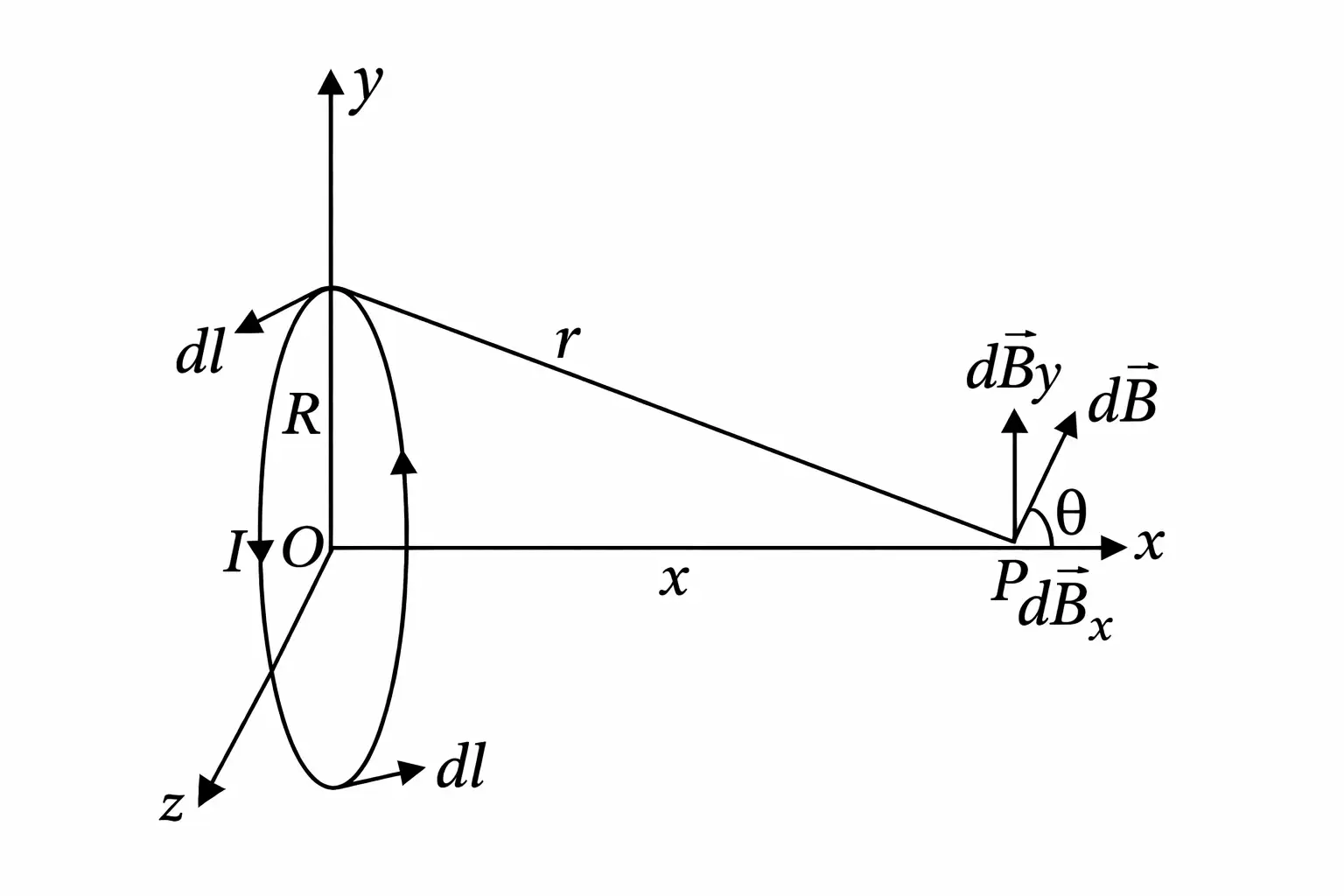
Integrating around the full loop uses .
Direction of the Field
- Right-hand rule: Curl the fingers of your right hand in the direction of current around the loop; your thumb points in the magnetic-field direction along the axis.
- Pole analogy: The face toward which the field points behaves like a north pole; the opposite face behaves like a south pole.
Special Cases
Set in the axial-field formula.
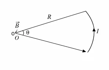
Field at the Centre of a Circular Arc
- Arc length: An arc of radius subtending angle at the centre has length , where is in radians.
- Field: The magnetic field at the centre due to the arc is .
Far from the Loop
- Condition: For , .
- Result: The axial field becomes , so .
- Interpretation: At large distances, a current loop behaves like a magnetic dipole.
State the magnetic field on the axis of a circular loop and its value at the centre.
What is the magnetic field at the centre due to a circular arc subtending angle ?
Quick recap
- The Biot–Savart law is .
- For a circular loop, transverse field components cancel and axial components add.
- The axial field is .
- At the centre of the loop, ; at the centre of an arc, .
- For , the field varies as and the loop behaves like a magnetic dipole.
Ampere’s Circuital Law
Ampere’s Circuital Law
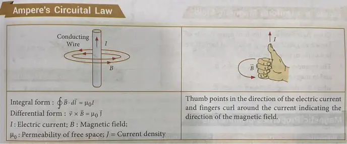
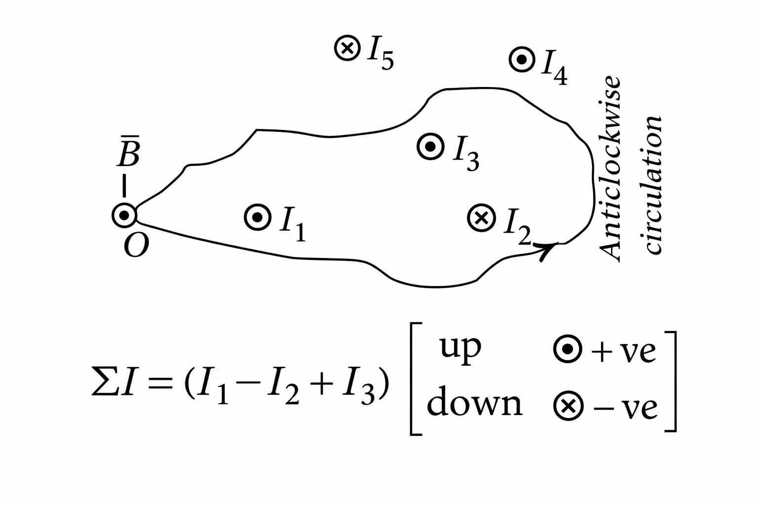
Applicability and Limitations
- Applicability: Ampere’s circuital law is especially useful for current distributions with sufficient symmetry to determine the magnetic field along a closed path.
- Thick conductors: Applying the law inside a thick wire requires its cross-sectional radius and current density.
- Current density: For the standard cylindrical-wire result, the current density is taken to be uniform across the cross-section.
Field of an Infinitely Long Solid Cylindrical Wire
Here is the wire’s cross-sectional area.
| Position | Enclosed current | Magnetic field | Variation |
|---|---|---|---|
| At the axis, | Zero | ||
| Inside the wire, | |||
| At the surface, | Maximum field | ||
| Outside the wire, |
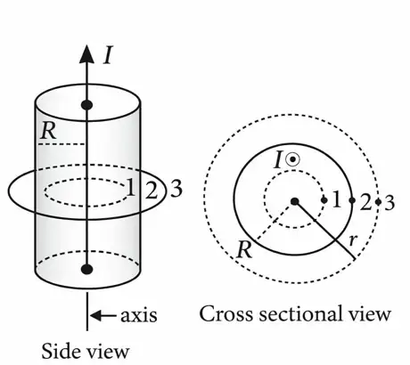
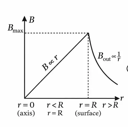
How does the magnetic field vary inside and outside a uniformly current-carrying solid cylindrical wire?
Quick recap
- Ampere’s law relates the closed-loop integral of the magnetic field to the net enclosed current.
- Choose an Amperian loop that matches the symmetry of the current distribution.
- A uniformly current-carrying solid wire has .
- Inside the wire, ; the field rises linearly with radius.
- At the surface, , its maximum value.
- Outside the wire, ; the field decreases as .
The Solenoid
Solenoid: construction and field
Solenoid — A solenoid is a coil whose length is much greater than its radius, used to produce a uniform magnetic field over a long range.
Construction and turn density
- Construction: A conducting wire is tightly wound in identical circular turns around a cylindrical frame.
- Axial field: The field at a point on the axis is obtained by superposing the fields from the circular turns.
- Turn density: For turns distributed over length , .
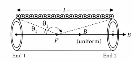
Here, is turns per unit length, is the current, and are the angles subtended by the solenoid ends at the field point.
Long and infinite solenoids
Magnetic field of an infinite solenoid
- Inside: The magnetic field is uniform and equals .
- Outside: The magnetic field outside an ideal infinite solenoid approaches zero.
- At the end: The field at an end is half the interior field.
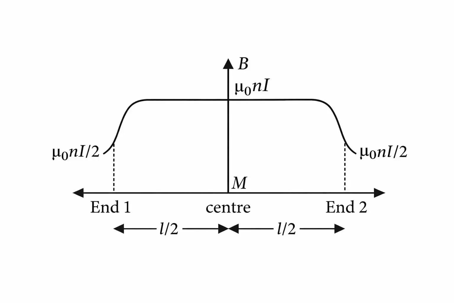
This is the approximately uniform interior field.
The field at the end is half the interior field.
For a frame with relative permeability , the interior field is multiplied by .
Quick recap
- A solenoid is a tightly wound cylindrical coil whose length greatly exceeds its radius, producing a uniform magnetic field over a long range.
- Turn density is .
- The finite-solenoid axial field is .
- An ideal infinite solenoid has uniform interior field ; its exterior field approaches zero.
- The field at an end is half the interior field: .
- With a magnetic frame, the field is .
Force Between Two Parallel Currents, the Ampere
Force Between Parallel Current-Carrying Wires
Mutual magnetic force
- Cause: Each wire lies in the magnetic field produced by the other, so each experiences a magnetic force.
- Direction: Currents in the same direction attract; currents in opposite directions repel.
- Field from wire 2 at wire 1: ; similarly, .
- Force on a length : The wire element is perpendicular to the other wire’s magnetic field.
For two long parallel wires separated by distance .
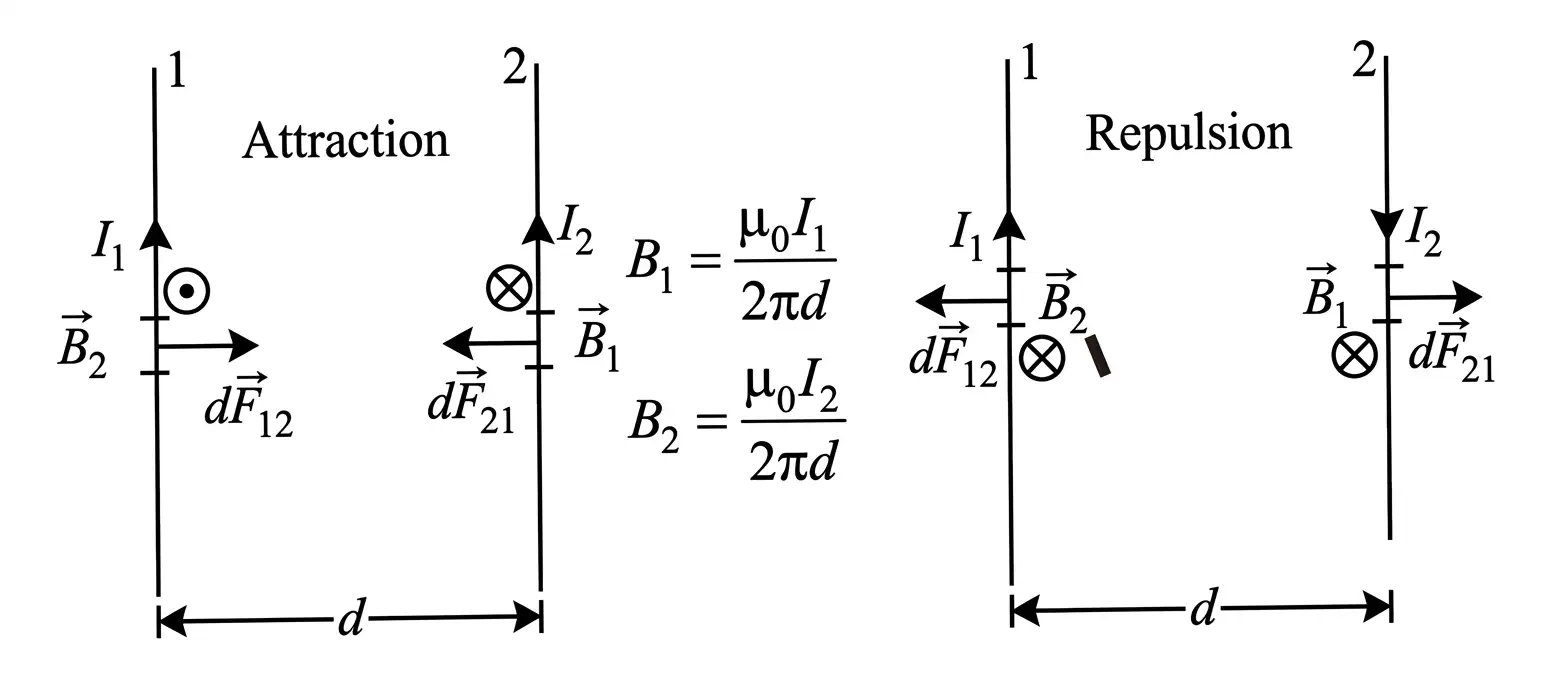
Definition of the Ampere
Ampere — One ampere is the current in each of two long, straight, parallel conductors apart in vacuum that produces a force of per metre between them.
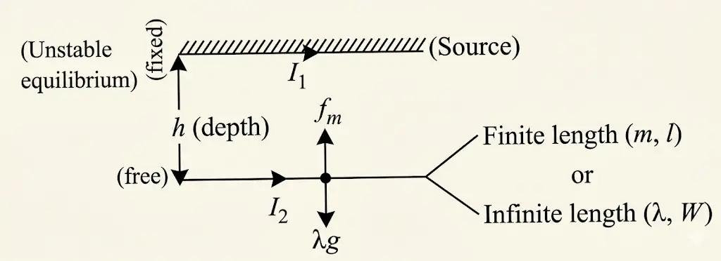
Application: Equilibrium of a Free Wire
Upper wire free
- Equilibrium: The magnetic force per unit length balances the wire’s weight per unit length at separation .
- Stable: A small vertical displacement produces a restoring force; the free wire oscillates in the vertical plane.
- Linear mass density: , so the weight per unit length is .
For small vertical oscillations of the stable upper wire.
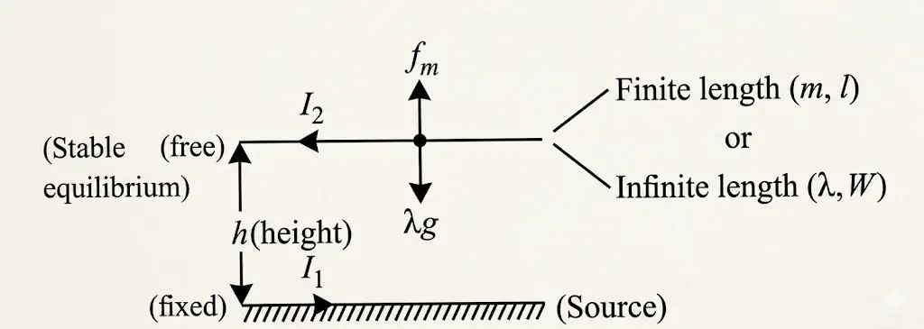
Lower wire free
- Equilibrium condition: The magnitudes of magnetic force and weight per unit length are equal, as for the upper wire.
- Unstable: A slight displacement makes the wire move farther from its equilibrium position—either upward or downward, depending on the displacement.
Quick recap
- Parallel currents in the same direction attract; currents in opposite directions repel.
- The force per unit length is .
- For equal currents of separated by in vacuum, the force per unit length is ; this defines the ampere in this setup.
- For either free-wire equilibrium at distance , .
- The upper free wire is stable and has small-oscillation period ; the lower free wire is unstable.
Torque on Current Loop, Magnetic Dipole
Torque on a Rectangular Current Loop
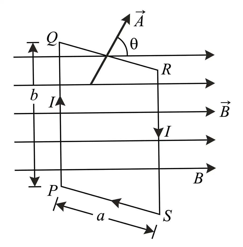
For identical turns, the torque is multiplied by .
Magnetic dipole moment — The magnetic dipole moment of a current loop is , directed along the area vector, normal to the loop’s plane.
The torque direction is given by the cross product of magnetic dipole moment and magnetic field.
Torque at special orientations
- Zero torque: If is parallel or antiparallel to , then or and ; the loop’s plane is normal to the field.
- Maximum torque: If , then ; the loop’s plane is parallel to the field.
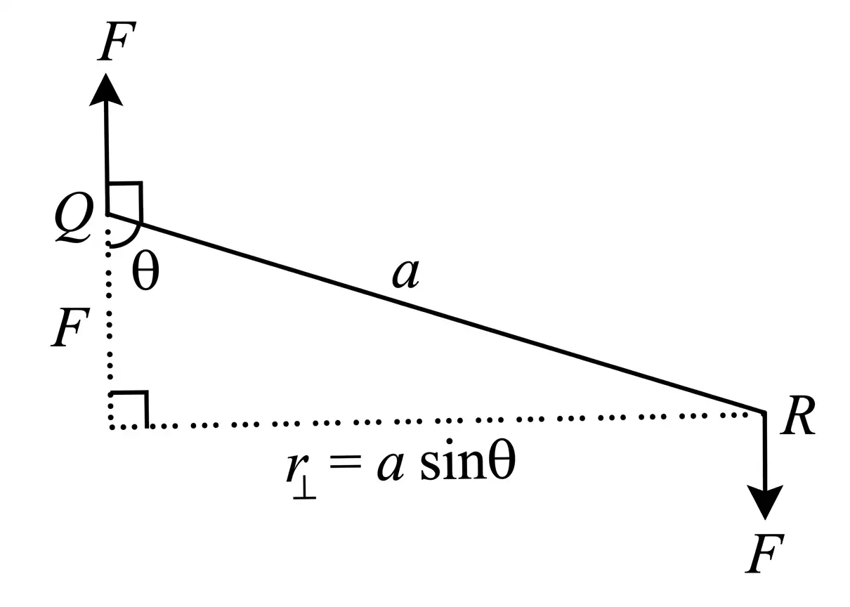
Do not confuse the loop’s plane with its area vector: when the plane is normal to , the area vector is parallel to and torque is zero.
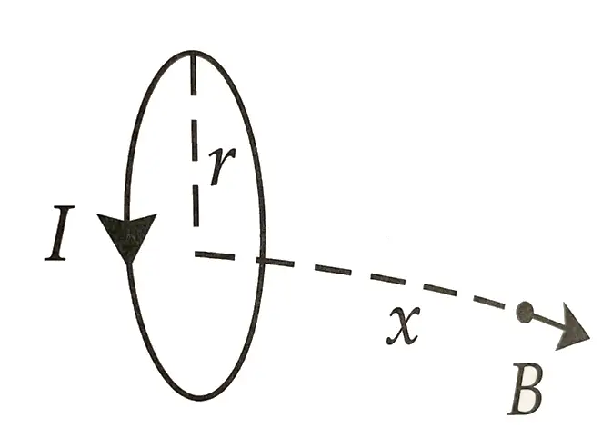
Circular Current Loop as a Magnetic Dipole
For a loop of radius carrying current , at an axial distance from its centre; .
For , the circular loop behaves like a magnetic dipole. For a single turn, .
Write the torque on an -turn current loop in a uniform magnetic field.
When is the torque on a current loop zero and when is it maximum?
Quick recap
- A current loop in a uniform magnetic field can experience torque because opposite forces may act along different lines.
- For an -turn loop, .
- The magnetic dipole moment is , and .
- Torque is zero when the area vector is parallel to the field and maximum when it is perpendicular.
- On the axis of a circular loop, the far-field strength decreases as and is .
The Moving Coil Galvanometer
Principle and working
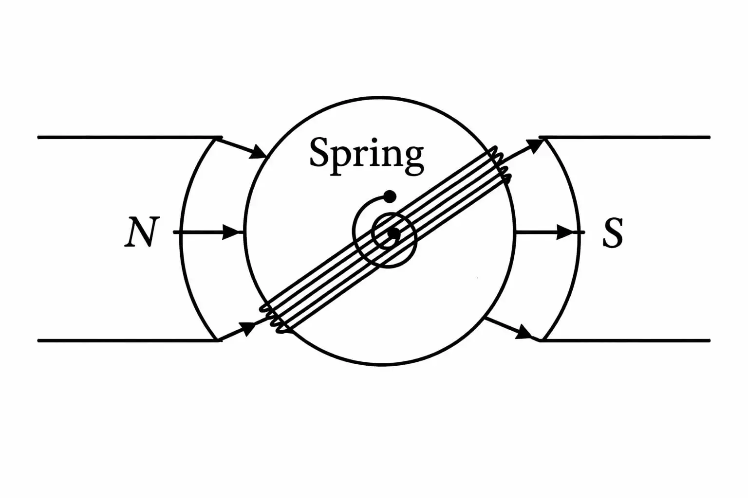
Deflection and galvanometer constant
Sensitivity
Deflection per unit current.
Deflection per unit potential difference, where .
Effect of increasing the number of turns
- Current sensitivity: Doubling doubles .
- Voltage sensitivity: If doubling also doubles the wire length and resistance , then does not change.
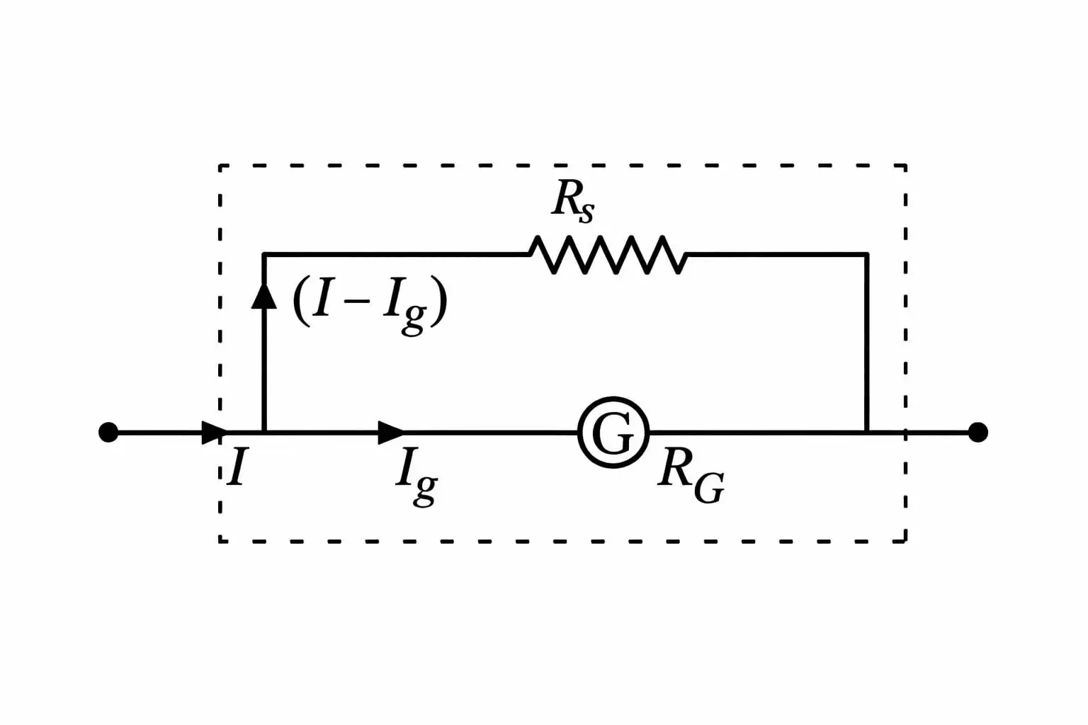
Conversion into an ammeter
Use this relation to choose the shunt for a desired ammeter range.
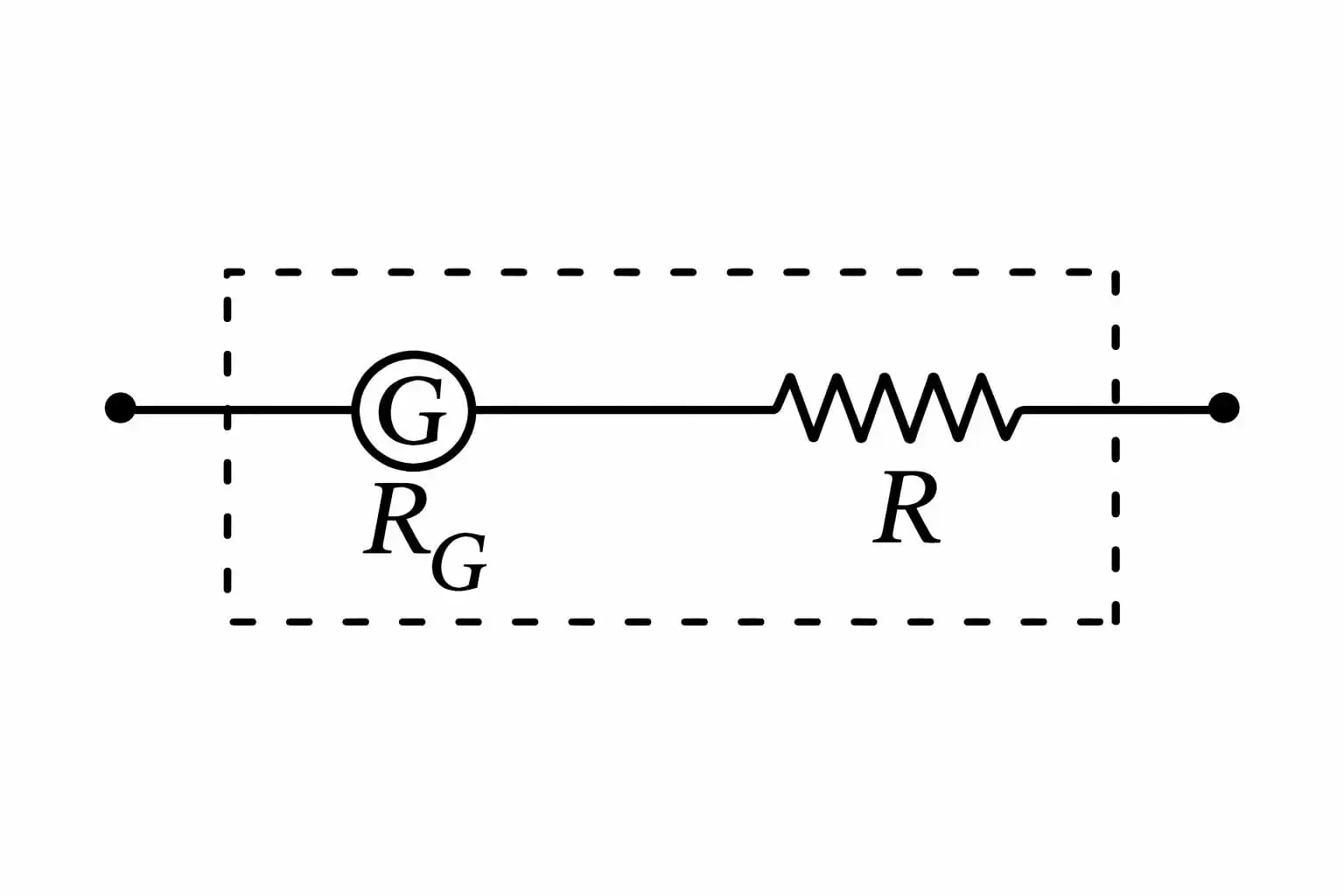
Conversion into a voltmeter
Quick recap
- A current-carrying coil in a magnetic field experiences torque; cylindrical pole pieces provide a radial field.
- At equilibrium, , so ; is the spring’s torsional constant.
- The galvanometer constant is ; current sensitivity is .
- Voltage sensitivity is and may stay unchanged if increased turns also increase resistance proportionally.
- A parallel shunt converts a galvanometer into an ammeter: .
- A large series resistance converts a galvanometer into a voltmeter: .
NEET Physics — ALL CHAPTERS
1
Basic Mathematics
2
Units and Measurement
3
Motion in a Straight Line
4
Motion in a Plane
5
Laws of Motion
6
Work, Energy and Power
7
System of Particles and Rotational Motion
8
Gravitation
9
Mechanical Properties of Solids
10
Mechanical Properties of Fluids
11
Thermal Properties of Matter
12
Thermodynamics
13
Kinetic Theory
14
Oscillations
15
Waves
16
Electric Charges and Fields
17
Electrostatic Potential and Capacitance
18
Current Electricity
19
Moving Charges and Magnetism
20
Magnetism and Matter
21
Electromagnetic Induction
22
Alternating Current
23
Electromagnetic Waves
24
Ray Optics and Optical Instruments
25
Wave Optics
26
Dual Nature of Radiation and Matter
27
Atoms
28
Nuclei
29
Semiconductor Electronics: Materials, Devices and Simple Circuits